Deep Learning with Minimal Training Data: TurkuNLP Entry in the BioNLP Shared Task 2016

Deep Learning with Minimal Training Data: TurkuNLP Entry in the

BioNLP Shared Task 2016

Farrokh Mehryary

_{, Jari Bj¨orne}

_{, Sampo Pyysalo}

_{, Tapio Salakoski}

_{and Filip Ginter}

_{University of Turku Graduate School (UTUGS)}

2

_{Turku Centre for Computer Science (TUCS)}

3

_{Department of Information Technology, University of Turku}

Faculty of Mathematics and Natural Sciences, FI-20014, Turku, Finland

4

_{Language Technology Lab, DTAL, University of Cambridge}

[email protected], [email protected]

Abstract

We present the TurkuNLP entry to the BioNLP Shared Task 2016 Bacte-ria Biotopes event extraction (BB3-event) subtask. We propose a deep learning-based approach to event extraction using a combination of several Long Short-Term Memory (LSTM) networks over syntac-tic dependency graphs. Features for the proposed neural network are generated based on the shortest path connecting the two candidate entities in the dependency graph. We further detail how this network can be efficiently trained to have good gen-eralization performance even when only a very limited number of training examples are available and part-of-speech (POS) and dependency type feature representa-tions must be learned from scratch. Our method ranked second among the entries to the shared task, achieving an F-score of 52.1% with 62.3% precision and 44.8% re-call.

1 Introduction

The BioNLP Shared Task 2016 was the fourth in the series to focus on event extraction, an infor-mation extraction task targeting structured asso-ciations of biomedical entities (Kim et al., 2009; Ananiadou et al., 2010). The 2016 task was also the third to include a Bacteria Biotopes (BB) sub-task focusing on microorganisms and their habi-tats (Bossy et al., 2011). Here, we present the TurkuNLP entry to the BioNLP Shared Task 2016 Bacteria Biotope event extraction (BB3-event) subtask. Our approach builds on proven tools and ideas from previous tasks and is novel in its ap-plication of deep learning methods to biomedical event extraction.

The BB task was first organized in 2011, then consisting of named entity recognition (NER) tar-geting mentions of bacteria and locations, fol-lowed by the detection of two types of relations involving these entities (Bossy et al., 2011). Three teams participated in this task, with the best F-score of 45% achieved by the INRA Bibliome group with the Alvis system, which used dic-tionary mapping, ontology inference and seman-tic analysis for NER, and co-occurrence-based rules for detecting relations between the entities (Ratkovic et al., 2011). The 2013 BB task de-fined three subtasks (N´edellec et al., 2013), the first one concerning NER, targeting bacteria habi-tat entities and their normalization, and the other two subtasks involving relation extraction, the task targeted also by the system presented here. Sim-ilarly to the current BB3-event subtask, the 2013 subtask 2 concerned only relation extraction, and subtask 3 extended this with NER. Four teams par-ticipated in these tasks, with the UTurku TEES system achieving the first places with F-scores of 42% and 14% (Bj¨orne and Salakoski, 2013).

We next present the 2016 BB3-event subtask and its data and then proceed to detail our method, its results and analysis. We conclude with a dis-cussion of considered alternative approaches and future work.

2 Task and Data

In this section, we briefly present the BB3-event task and the statistics of the data that has been used for method development and optimization, as well as for test set prediction.

ex-Train Devel Test

Total sentences 527 319 508

Sentences w/examples 158 117 158

Sentences w/o examples 369 202 350

Total examples 524 506 534

Positive examples 251 177

-Negative examples 273 329

-Table 1: BB3-event data statistics. (The relation annotations of the test set have not been released.)

clusively marking directed binary associations of exactly two entities. For the purposes of machine learning, we thus cast the BB3-event task as binary classification taking either a (BACTERIA, HABI -TAT) or a (BACTERIA, GEOGRAPHICAL) entity

pair as input and predicting whether or not a Lives-in relation holds between the BACTERIA and the

location (HABITATor GEOGRAPHICAL).

Our approach builds on the shortest dependency path between each pair of entities. However, while dependency parse graphs connect words to oth-ers in the same sentence, a number of annotated relations in the data involve entities appearing in different sentences, where no connecting path ex-ists. Such cross-sentence associations are known to represent particular challenges for event extrac-tion systems, which rarely attempt their extracextrac-tion (Kim et al., 2011). In this work, we simply ex-clude cross-sentence examples from the data. This elimination procedure resulted in the removal of 106 annotated relations from the training set and 62 annotated relations from the development set.

The examples that we use for the training, optimization and development evaluation of our method are thus a subset of those in the origi-nal data.1 _{When discussing the training,} develop-ment and test data, we refer to these filtered sets throughout this manuscript. The statistics of the task data after this elimination procedure are sum-marized in Table 1. Note that since there are var-ious ways of converting the shared task annota-tions into examples for classification, the numbers we report here may differ from those reported by other participating teams.

1_{Official evaluation results on the test data are of course}

comparable to those of other systems: any cross-sentence re-lations in the test data count against our submission as false negatives.

3 Method

We next present our method in detail. Preprocess-ing is first discussed in Section 3.1. Section 3.2 then explains how the shortest dependency path is used, and the architecture of the proposed deep neural network is presented in Section 3.3. Sec-tion 3.4 defines the classificaSec-tion features and em-beddings for this network. Finally, in Section 3.5 we discuss the training and regularization of the network.

3.1 Preprocessing

We use the TEES system, previously developed by members of the TurkuNLP group (Bj¨orne and Salakoski, 2013), to run a basic preprocessing pipeline of tokenization, POS tagging, and pars-ing, as well as to remove cross-sentence relations. Like our approach, TEES targets the extraction of associations between entities that occur in the same sentence. To support this functionality, it can detect and eliminate relations that cross sen-tence boundaries in its input. We use this feature of TEES as an initial preprocessing step to remove such relations from the data.

To obtain tokens, POS tags and parse graphs, TEES uses the BLLIP parser (Charniak and John-son, 2005) with the biomedical domain model cre-ated by McClosky (2010). The phrase structure trees produced by the parser are further processed with the Stanford conversion tool (de Marneffe et al., 2006) to create dependency graphs. The Stan-ford system can produce several variants of the Stanford Dependencies (SD) representation. Here, we use thecollapsedvariant, which is designed to be useful for information extraction and language understanding tasks (de Marneffe and Manning, 2008).

3.2 Shortest Dependency Path

The syntactic structure connecting two entitiese1

and e2 in various forms of syntactic analysis is

known to contain most of the words relevant to characterizing the relationship R(e1, e2), while

ex-tracting features (Bj¨orne et al., 2012; Bj¨orne and Salakoski, 2013). Recently, this idea was applied in an LSTM-based relation extraction system by Xu et al. (2015). Since the dependency parse is di-rected (i.e. the path frome1toe2differs from that

from e2 to e1), they separate the shortest

depen-dency path into two sub-paths, each from an entity to the common ancestor of the two entities, gen-erate features along the two sub-paths, and feed them into different LSTM networks, to process the information in a direction sensitive manner.

To avoid doubling the number of LSTM chains (and hence the number of weights), we convert the dependency parse to an undirected graph, find the shortest path between the two entities (BACTERIA

and HABITAT/GEOGRAPHICAL), and always

pro-ceed from the BACTERIA entity to the HABI -TAT/GEOGRAPHICALentity when generating

fea-tures along the shortest path, regardless of the or-der of the entity mentions in the sentence. With this approach, there is a single LSTM chain (and set of LSTM weights) for every feature set, which is more effective when the number of training ex-amples is limited.

There is a subtle and important point to be addressed here: as individual entity mentions can consist of several (potentially discontinu-ous) tokens, the method must be able to select which word (i.e. single token) serves as the start-ing/ending point for paths through the dependency graph. For example, in the following training set sentence, “biotic surfaces”is annotated as a HABITATentity:

“We concluded that S. marcescens MG1 utilizes different regulatory systems and adhesins in attachment to biotic and abioticsurfaces[...]”

As this mention consists of two (discontinuous) tokens, it is necessary to decide whether the paths connecting this entity to BACTERIA

men-tions (e.g., “S. marcescens MG1”) should end at

“biotic” or“surfaces”. This problem has fortu-nately been addressed in detail in previous work, allowing us to adopt the proven solution proposed by Bj¨orne et al. (2012) and implemented in the TEES system, which selects the syntactic head, i.e. the root token of the dependency parse sub-tree covering the entity, for any given multi-token en-tity. Hence, in the example above, the token “sur-faces”is selected and used for finding the shortest dependency paths.

3.3 Neural Network Architecture

While recurrent neural networks (RNNs) are in-herently suitable for modeling sequential data, standard RNNs suffer from the vanishing or ex-ploding gradientsproblem: if the network is deep, during the back-propagation phase the gradients may either decay exponentially, causing learning to become very slow or stop altogether ( vanish-inggradients); or become excessively large, caus-ing the learncaus-ing to diverge (exploding gradients) (Bengio et al., 1994). To avoid this issue, we make use of Long Short-Term Memory (LSTM) units, which were proposed to address this prob-lem (Hochreiter and Schmidhuber, 1997).

We propose an architecture centered around three RNNs (chains of LSTM units): one rep-resenting words, the second POS tags, and the third dependency types (Figure 1). For a given example, the sequences of words, POS tags and dependency types on the shortest dependency path from the BACTERIA mention to the HABI -TAT/GEOGRAPHICAL mention are first mapped

into vector sequences by three separate embedding lookup layers. These word, POS tag and depen-dency type vector sequences are then input into the three RNNs. The outputs of the last LSTM unit of each of the three chains are then concate-nated and the resulting higher-dimensional vector input to a fully connected hidden layer. The hid-den layer finally connects to a single-node binary classification layer.

Based on experiments on the development set, we have set the dimensionality of all LSTM units and the hidden layer to 128. The sigmoid activa-tion funcactiva-tion is applied on the output of all LSTM units, the hidden layer and the output layer.

3.4 Features and Embeddings

We next present the different embeddings defining the primary features of our model. In addition to the embeddings, we use a binary feature which has the value0if the corresponding location is a GEO -GRAPHICALentity and1if it is a HABITATentity.

This input is directly concatenated with the LSTM outputs and fed into the hidden layer. We noticed this signal slightly improves classification perfor-mance, resulting in a less than 1 percentage point increase of the F-score.

3.4.1 Word embeddings

detection NN products NNS

Salmonellae NNP nn prep_in

detection products NNP NN NNS nn prep_in

Concatenate

Fully connected

Fully connected RNNs Embedding Inputs

Shortest path

+ target type Habitat

Salmonellae

words parts of speech dependencies

Figure 1: Proposed network architecture.

scientific text, namely the combined texts of all PubMed titles and abstracts and PubMed Central Open Access (PMC OA) full text articles avail-able as of the end of September 2013.2 _These 200-dimensional vectors were created by Pyysalo et al. (2013) using theword2vecimplementation of theskip-grammodel (Mikolov et al., 2013).

To reduce the memory requirements of our method, we only use the vectors of the 100,000 most frequent words to construct the embedding matrix. Words not included in this vocabulary are by default mapped to a shared, randomly ini-tialized unknown word vector. As an exception, out of vocabulary BACTERIAmentions are instead

mapped to the vector of the word “bacteria”. Based on development set experiments we esti-mate that this special-case processing improved the F-score by approximately 1% point.

3.4.2 POS embeddings

Our POS embedding matrix consists of a 100-dimensional vector for each of the POS tags in the Penn Treebank scheme used by the applied tagger. We do not use pre-trained POS vectors but instead initialize the embeddings randomly at the begin-ning of the traibegin-ning phase.

2_{Available fromhttp://bio.nlplab.org/}

3.4.3 Dependency type embeddings

Typed dependencies – the edges of the parse graph – represent directed grammatical relations between the words of a sentence. The sequence of dependencies on the shortest path between two entities thus conveys highly valuable information about the nature of their relation.

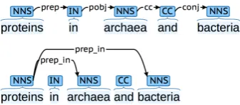
We map each dependency type in the collapsed SD representation into a randomly initialized 350-dimensional vector (size set experimentally). Note that in the applied SD variant, prepositions and conjunctions become part of collapsed depen-dency types (de Marneffe et al., 2006), as illus-trated in Figure 2.

Figure 2: Basic (top) and collapsed (bottom) Stan-ford Dependency representations

develop-ment sets are mapped to the vectors for the gen-eral preposition and conjunction typesprepand

conj, respectively.

3.5 Training and Regularization

We usebinary cross-entropyas the objective func-tion and theAdamoptimization algorithm with the parameters suggested by Kingma and Ba (2014) for training the network. We found that this al-gorithm yields considerably better results than the conventional stochastic gradient descent in terms of classification performance.

During training, the randomly initialized POS and dependency type embeddings are trained and the pre-trained word embeddings fine-tuned by back-propagation using the supervised signal from the classification task at hand.

Determining how long to train a neural network model for is critically important for its generaliza-tion performance. If the network isunder-trained, model parameters will not have converged to good values. Conversely, over-training leads to over-fitting on the training set. A conventional solu-tion is early stopping, where performance is eval-uated on the development set after each set pe-riod of training (e.g. one pass through the train-ing set, or epoch) to decide whether to continue or stop the training process. A simple rule is to continue while the performance on the develop-ment set is improving. By repeating this approach for 15 different runs with different initial ran-dom initializations of the model, we experimen-tally concluded that the optimal length of training is four epochs. Overfitting is a serious problem in deep neural networks with a large number of pa-rameters. To reduce overfitting, we experimented with several regularization methods including the

l1 weight regularization penalty (LASSO) and the l2weight decay (ridge) penalty on the hidden layer

weights. We also tried the dropout method (Srivas-tava et al., 2014) on the output of LSTM chains as well as on the output of the hidden layer, with a dropout rate of 0.5. Out of the different combi-nations, we found the best results when applying dropout after the hidden layer. This is the only regularization method used in the final method.

4 Results

4.1 Overcoming Variance

At the beginning of training, the weights of the neural network are initialized randomly. As we are

Run Recall Precision F-score

12 76.3 60.3 _67.3

14 71.2 63.0 66.8

13 75.7 59.3 _66.5

10 78.0 56.3 65.4

3 80.8 54.0 64.7

15 79.1 54.3 _64.4

1 66.1 62.2 64.1

11 65.0 62.8 _63.9

2 67.8 59.4 _63.3

5 55.9 69.7 62.1

7 57.6 66.7 _61.8

9 53.1 70.2 60.5

8 50.9 74.4 _60.4

6 50.3 73.6 _59.7

4 46.9 78.3 58.7

¯

x 65.0 64.3 63.3

σ 11.3 7.3 _2.6

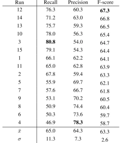
Table 2: Development set results for 15 repeti-tions with different initial random initializarepeti-tions with mean (¯x) and standard deviation (σ). Results are sorted by F-score.

only using pre-trained embeddings for words, this random initialization applies also to the POS and dependency type embeddings. Since the number of weights is high and the training set is very small (only 524 examples), the initial random state of the model can have a significant impact on the final model and its generalization performance. Lim-ited numbers of training examples are known to represent significant challenges for leveraging the full power of deep neural networks, and we found this to be the case also in this task.

Threshold (t) Recall Precision F-score

1 83.6 53.2 _65.1

2 79.7 54.0 64.4

3 78.5 57.0 _66.0

4 78.0 59.0 67.2

5 75.7 60.1 67.0

6 70.6 60.7 _65.3

7 67.8 61.5 64.5

8 65.5 62.0 _63.7

9 62.2 65.5 _63.8

10 58.2 66.5 62.1

11 57.1 69.7 _62.7

12 52.5 70.5 60.2

13 51.4 72.8 _60.3

14 48.6 74.8 _58.9

15 45.2 80.0 57.8

Table 3: Development set results for voting based on the predictions of the 15 different classifiers. Best results for each metric shown in bold.

set, individual models that achieved high perfor-mance in this experiment will not necessarily gen-eralize well to unseen data.

To deal with these issues, we introduce a straightforward voting procedure that aggregates the prediction outputs of the 15 classifiers based on a given threshold valuet∈ {1, . . . ,15}:

1. For each example, predict outputs with the 15 models;

2. If at leasttoutputs are positive, label the ex-ample positive, otherwise label it negative. Clearly, the most conservative threshold ist= 15, where a relation is voted to exist only ifallthe 15 classifiers have predicted it. Conversely, the least conservative threshold ist= 1, where a relation is voted to hold ifanyclassifier has predicted it.

The development set results for the voting al-gorithm with different threshold values are given in Table 3. As expected, the threshold t = 1 produces the highest recall (83.6%) with the low-est precision (53.2%). With increasing values of

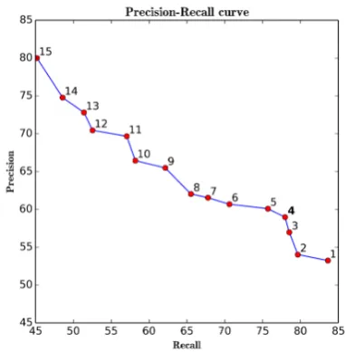
t, precision increases while recall drops, and the highest precision (80.0%) is achieved together the lowest recall of (45.2%) with t = 15. The best F-score is obtained witht= 4, where an example is labeled positive if at least four classifiers have predicted it to be positive and negative otherwise. Figure 3 shows the precision-recall curve for these 15 threshold values.

Figure 3: Precision-recall curve for different val-ues of the threshold t (shown as labels on the curve).

As is evident from these results, the voting al-gorithm can be used for different purposes. If the aim is to obtain the best overall performance, we can investigate which threshold produces the high-est F-score (heret= 4) and select that value when making predictions for unseen data (e.g., the test set). Alternatively, for applications that specifi-cally require high recall or high precision, a dif-ferent threshold value can be selected to optimize the desired metric.

To assess the performance of the method on the full, unfiltereddevelopment set that includes also cross-sentence relations, we selected the threshold valuet= 4and submitted the aggregated predic-tion results to the official Shared Task evaluapredic-tion server. The method achieved an F-score of 60.0% (60.9% precision and 59.3% recall), 7.2% points below the result for our internal evaluation with filtered data (Table 3).

4.2 Test Set Evaluation

Our method achieved an F-score of 52.1% with a recall of 44.8% and precision of 62.3%, rank-ing second among the entries to the shared task. We again emphasize that our approach ignored all potential relations between entities belonging to different sentences, which may in part explain the comparatively low recall.

4.3 Runtime Performance and Technical Details

We implemented the model using the Python pro-gramming language (v2.7) with Keras, a model-level deep learning library (Chollet, 2015). All network parameters not explicitly discussed above were left to their defaults in Keras. The Theano tensor manipulation library (Bastien et al., 2012) was used as the backend engine for Keras. Com-putations were run on a single server computer equipped with a GPU.3_{All basic python} process-ing, including e.g. file manipulation, the TEES pipeline and our voting algorithm, was run on a single CPU core, while all neural network related calculations (training, optimization, predictions) were run on the GPU, using the CUDA toolkit ver-sion 5.0.

The training process takes about 10 minutes, in-cluding model building and 4 epochs of training the network on the training set, but excluding pre-processing and the creation and loading of the in-put network. Prediction of the development set using a trained model with fully prepared inputs is very fast, taking only about 10 seconds. Finally, the voting algorithm executes in less than a minute for all 15 thresholds.

We note that even though the proposed ap-proach involving 15 rounds of training, predic-tion and result aggregapredic-tion might seem to be impractical for large-scale real-word applications (e.g., extracting bacteria-location relations from all PubMed abstracts), it is quite feasible in prac-tice, as the time-consuming training process only needs to be done once, and prediction on unseen data is quite fast.

4.4 Other Architectures

In this section, we discuss alternative approaches that we considered and the reasons why they were rejected in favor of that described above.

3_{In detail: two 6-core Intel}R _XeonR _{E5-2620processors,} 32 gigabytes of main memory, and one NVIDIAR _TESLATM C2075companion processor with 448 CUDA cores and 6 gi-gabytes of memory.

One popular and proven method for relation extraction is to use three groups of features, based on the observation that the words preceding the first entity, the words between the entities, and those after the second entity serve different roles in deciding whether or not the entities are related (Bunescu and Mooney, 2006). Given a sentence S=w1, ..., e1, ..., wi, ..., e2, ..., wn

with entities e1 and e2, one can represent

the sentence with three groups of words: {before}e1{middle}e2{after} (e1 and e2 can

also be included in the groups). The similarity of two examples represented in this way can be compared using e.g.sub-sequence kernelsat word level (Bach and Badaskar, 2007). Bunescu and Mooney (2006) utilize three subkernels matching combinations of the before, middle and after sequences of words, with a combined kernel that is simply the sum of the subkernels. This kernel is then used with support vector machines for rela-tion extracrela-tion. Besides the words, other features such as the corresponding POS tags and entity types can also be incorporated into such kernel functions to further improve the representation.

We adapted this idea to deep neural networks. We started with the simplest architecture, which contains 3 LSTM networks. Instead of gener-ating features based on the shortest path, each LSTM receives inputs based on the sequence of the words seen in each of thebefore,middle, and

after groups, where the word embeddings are the only features used for classification. Similar to the architecture discussed in Section 3.3, the outputs of the last LSTM units in each chain are concate-nated, and the resulting higher-dimensional vector is then fed into a fully connected hidden layer and then to the output layer. This approach has a ma-jor advantage over the shortest dependency path, in particular for large-scale applications: parsing,

the most time-consuming part in the relation ex-traction pipeline, is no longer required.

that even though not requiring parsing is a benefit in these approaches, our experiments suggest that they are not capable of reaching performance com-parable to methods that use the syntactic structure of sentences.

5 Conclusions and Future work

We have presented the entry of the TurkuNLP team to the Bacteria Biotope event extraction (BB3-event) sub-task of the BioNLP Shared Task 2016. Our method is based on a combination of LSTM networks over syntactic dependency graphs. The features for the network are derived from the POS tags, dependency types, and word forms occurring on the shortest dependency path connecting the two candidate entities (BACTERIA

and HABITAT/GEOGRAPHICAL) in the collapsed

Stanford Dependency graph.

We initialize word representations using pre-trained vectors created using six billion words of biomedical text (PubMed and PMC documents). During training, the pre-trained word embeddings are fine-tuned while randomly initialized POS and dependency type representations are trained from scratch. We showed that as the number of train-ing examples is very limited, the random initial-ization of the network can considerably impact the quality of the learned model. To address this issue, we introduced a voting approach that ag-gregates the outputs of differently initialized neu-ral network models. Different aggregation thresh-olds can be used to select different precision-recall trade-offs. Using this method, we showed that our proposed deep neural network can be effi-ciently trained to have good generalization for un-seen data even with minimal training data. Our method ranked second among the entries to the shared task, achieving an F-score of 52.1% with 62.3% precision and 44.8% recall.

There are a number of open questions regard-ing our model that we hope to address in future work. First, we observed how the initial random state of the model can impact its final performance on unseen data. It is interesting to investigate whether (and to what extent) pre-training the POS and dependency type embeddings can address this issue. One possible approach would be to ap-ply the method to similar biomedical relation ex-traction tasks that include larger corpora than the BB3-event task (Pyysalo et al., 2008) and use the learned POS and dependency embeddings for

ini-tialization for this task. This could also establish to what extent pre-training these representations can boost the F-score.

Second, it will be interesting to study how the method performs with different amounts of train-ing data. On one hand, we can examine to what extent the training corpus size can be reduced without compromising the ability of the proposed network to learn the classification task; on the other, we can explore how this deep learning method compares with previously proposed state-of-the-art biomedical relation extraction methods on larger relation extraction corpora.

Third, the method and task represent an oppor-tunity to study how the word embeddings used for initialization impact relation extraction perfor-mance and in this way assess the benefits of dif-ferent methods for creating word embeddings in an extrinsic task with real-world applications.

Finally, it is interesting to investigate differ-ent methods to deal with cross-sdiffer-entence relations. Here we ignored all potential relations where the entities are mentioned in different sentences as there is no path connecting tokens across sen-tences in the dependency graph. One simple method that could be considered is to create an artificial “paragraph” node connected to all sen-tence roots to create such paths (cf. e.g. Melli et al. (2007)).

We aim to address these open questions and fur-ther extensions of our model in future work.

Acknowledgments

We would like to thank Kai Hakala, University of Turku, for his technical suggestions for the pipeline development and the anonymous review-ers for their insightful comments and suggestions. We would also like to thank the CSC IT Center for Science Ltd. for computational resources. This work has been supported in part by Medical Re-search Council grant MR/M013049/1.

References

Antti Airola, Sampo Pyysalo, Jari Bj¨orne, Tapio Pahikkala, Filip Ginter, and Tapio Salakoski. 2008. All-paths graph kernel for protein-protein interac-tion extracinterac-tion with evaluainterac-tion of cross-corpus learn-ing. BMC bioinformatics, 9(11):1.

sys-tems biology by text mining the literature.Trends in biotechnology, 28(7):381–390.

Nguyen Bach and Sameer Badaskar. 2007. A review of relation extraction.Language Technologies Insti-tute, Carnegie Mellon University.

Fr´ed´eric Bastien, Pascal Lamblin, Razvan Pascanu, James Bergstra, Ian J. Goodfellow, Arnaud Berg-eron, Nicolas Bouchard, and Yoshua Bengio. 2012. Theano: new features and speed improvements. InProc. Deep Learning and Unsupervised Feature Learning NIPS 2012 Workshop.

Yoshua Bengio, Patrice Simard, and Paolo Frasconi. 1994. Learning long-term dependencies with gradi-ent descgradi-ent is difficult. IEEE Transactions on Neu-ral Networks, 5(2):157–166.

Jari Bj¨orne and Tapio Salakoski. 2013. TEES 2.1: Au-tomated annotation scheme learning in the bionlp 2013 shared task. In Proc. BioNLP Shared Task, pages 16–25.

Jari Bj¨orne, Filip Ginter, and Tapio Salakoski. 2012. University of Turku in the BioNLP’11 shared task.

BMC Bioinformatics, 13(S-11):S4.

Robert Bossy, Julien Jourde, Philippe Bessi`eres, Maarten van de Guchte, and Claire N´edellec. 2011. Bionlp shared task 2011: Bacteria biotope. InProc. BioNLP Shared Task, pages 56–64.

Razvan C. Bunescu and Raymond J. Mooney. 2005. A shortest path dependency kernel for relation extrac-tion. InProc. HLT-EMNLP, pages 724–731. Razvan Bunescu and Raymond J. Mooney. 2006.

Sub-sequence kernels for relation extraction. In Proc. NIPS.

Eugene Charniak and Mark Johnson. 2005. Coarse-to-fine N-best parsing and maxent discriminative reranking. InProc. ACL, pages 173–180.

Franois Chollet. 2015. Keras. https://github. com/fchollet/keras.

Faisal Mahbub Chowdhury, Alberto Lavelli, and Alessandro Moschitti. 2011. A study on de-pendency tree kernels for automatic extraction of protein-protein interaction. InProc. BioNLP 2011, pages 124–133.

Marie-Catherine de Marneffe and Christopher D. Man-ning. 2008. The stanford typed dependencies repre-sentation. InProc. CrossParser, pages 1–8. Marie-Catherine de Marneffe, Bill MacCartney, and

Christopher D. Manning. 2006. Generating typed dependency parses from phrase structure parses. In

Proc. LREC-2006, pages 449–454.

Sepp Hochreiter and J¨urgen Schmidhuber. 1997. Long short-term memory. Neural Comput., 9(8):1735– 1780.

Jin-Dong Kim, Tomoko Ohta, Sampo Pyysalo, Yoshi-nobu Kano, and Jun’ichi Tsujii. 2009. Overview of BioNLP’09 shared task on event extraction. InProc. BioNLP Shared Task, pages 1–9.

Jin-Dong Kim, Tomoko Ohta, Sampo Pyysalo, Yoshi-nobu Kano, and Junichi Tsujii. 2011. Ex-tracting bio-molecular events from literature - the BioNLP’09 shared task. Computational Intelli-gence, 27(4):513–540.

Diederik P. Kingma and Jimmy Ba. 2014. Adam: A method for stochastic optimization. CoRR, abs/1412.6980.

David McClosky. 2010. Any Domain Parsing: Au-tomatic Domain Adaptation for Natural Language Parsing. Ph.D. thesis.

Gabor Melli, Martin Ester, and Anoop Sarkar. 2007. Recognition of multi-sentence n-ary subcellular lo-calization mentions in biomedical abstracts. In Pro-ceedings of LBM.

Tomas Mikolov, Ilya Sutskever, Kai Chen, Greg S Cor-rado, and Jeff Dean. 2013. Distributed representa-tions of words and phrases and their compositional-ity. InAdvances in Neural Information Processing Systems 26, pages 3111–3119.

Claire N´edellec, Robert Bossy, Jin-Dong Kim, Jung-Jae Kim, Tomoko Ohta, Sampo Pyysalo, and Pierre Zweigenbaum. 2013. Overview of BioNLP shared task 2013. InProc. BioNLP Shared Task, pages 1–7. Truc-Vien T Nguyen, Alessandro Moschitti, and Giuseppe Riccardi. 2009. Convolution kernels on constituent, dependency and sequential structures for relation extraction. In Proc. EMNLP, pages 1378–1387.

Sampo Pyysalo, Antti Airola, Juho Heimonen, Jari Bj¨orne, Filip Ginter, and Tapio Salakoski. 2008. Comparative analysis of five protein-protein interac-tion corpora. BMC bioinformatics, 9(3):1.

Sampo Pyysalo, Filip Ginter, Hans Moen, Tapio Salakoski, and Sophia Ananiadou. 2013. Distribu-tional semantic resources for biomedical text min-ing. InProc. LBM, pages 39–44.

Zorana Ratkovic, Wiktoria Golik, Pierre Warnier, Philippe Veber, and Claire N´edellec. 2011. BioNLP 2011 task Bacteria Biotope: The Alvis system. In

Proc. BioNLP Shared Task, pages 102–111. Nitish Srivastava, Geoffrey Hinton, Alex Krizhevsky,

Ilya Sutskever, and Ruslan Salakhutdinov. 2014. Dropout: A simple way to prevent neural networks from overfitting. Journal of Machine Learning Re-search, 15:1929–1958.