Munich Personal RePEc Archive
A weighted location differential tax
method in environmental problems
Halkos, George and Kitsou, Dimitra
Department of Economics, University of Thessaly
26 October 2014
1
A weighted location differential tax method in
environmental problems
George E. Halkos
and Dimitra C. Kitsou
Laboratory of Operations Research, Department of Economics,
University of Thessaly
Abstract
Relying on Pigou's view, environmental taxes increase the costs of polluting activities reflecting in this way the true social cost imposed to society by the caused environmental damage by these activities. The total pollution cost (TPC) is defined by adding up the marginal abatement (MAC) and the marginal damage (MD) costs. That is the random variable TPC includes the social costs associated with pollution. We relate this with contaminated locations and propose a weighted location differentiated tax and a corresponding index that adjusts taxation to the damages caused. It is clear that the value of the expected total pollution (social) cost, E(TPC), would be of interest and therefore we proceed to the evaluation through the use of the γ)order Generalized Normal. The value of the variance, Var(TPC), is also evaluated and we provide a generalized form of the E(TPC) as far (i) the form of TPC and (ii) the probability density function.
Keywords: Weighted)location adjusted differential tax; pollution related social cost; expected value; technology;probability density function.
Keywords: C02; C60; Q50; Q53; Q58.
__________________________________________________________
2
1. Introduction
In the past, command and control regulations (like limiting the use of specific
fuels or demanding certain pollution sources to use specific methods) dominated
environmental policies with market based instruments (like taxes and tradable
permits) to dominate over the last decades. Environmental taxation relies on Pigou’s
concept of increasing polluters’ private costs to a level that includes the associated
true social costs imposed to the society by their activities and the resulting related
environmental damages.
Economic theory indicates that the optimal tax rate is determined where
marginal abatement cost (MAC) equals to marginal damage cost (MD) of pollution to
be abated. In a first best policy taxes should be differentiated between pollution
sources according to the size of their resulting damage costs. A second best policy
relies on the imposition of a high uniform tax rate. Halkos (1993) showed that moving
from the first best optimum to a uniform tax rate does make a difference. Specifically
and in the case of the acid rain problem in Europe it was shown that the costs of
moving from the first)best to the imposition of a high uniform tax rate may not differ
so much across countries but may be quite different within countries.
Pollution control and damage cost functions are non)linear and their exact
shapes are usually unknown (Halkos and Kitsos, 2005; Halkos and Kitsou, 2014). At
the same time, environmental effects are associated with significant irreversibilities
interacting often in a very complex way with uncertainty. This complexity becomes
even worse when taking into account the very long)run character of many
environmental problems. Uncertainties in abatement and damage cost functions affect
policy design in various ways. When marginal abatement costs are known and
3
authorities) can minimize social cost by introducing a pollution tax that equalizes
marginal abatement and damage costs.
But firms do not have always an incentive to reveal their true abatement
costs.1 A weighted location adjusted differentiated taxation is introduced, based on the
principle that when pollution is above “an optimal and accepted level” more taxation
has to be imposed, while if it is below there is a chance of less taxation. In this way a
new index to adjust taxation to the damage caused is proposed.
In the absence of information about costs, the level of emissions taxes needed
to achieve a target level of pollution abatement is unknown. This problem can be
overcome by using an iterative procedure in which tax is adjusted. The tax that its tax
system results in the social optimal pollution level is the differential tax. With
differential taxation, the marginal emission tax paid by firm i is always equal to
marginal damage costs and thereby minimizing social costs. The reason why this tax
system results in the social optimal pollution level is that the firms )faced with a tax
level that depends on emissions of firms) have an incentive to share information with
respect to their abatement cost.
The analysis becomes more complicated when the abatement costs are
stochastic, i.e. developed around it a probabilistic randomness. In this case or when
we have changes in the marginal abatement costs, specific environmental policies are
required, because the results from the changes of the Pigouvian taxation may be
1
4
considered obsolete. Marginal abatement costs may change over time, by changing
the innovative standards in the industry and by adopting the rapidly evolving new
technologies. It is worth mentioning that adoption of new technologies reduces or
aims to reduce emissions.
Given innovation outcome (X), the Total Pollution Cost (TPC) is defined by
the sum of the marginal abatement (MAC) and the marginal damage (MD) costs. That
is the random variable TPC includes the social costsassociated with pollution. In this
paper we evaluate the expected value of TPC and introduce the estimation of its
variance. Specifically, choosing as TPC the general form TPC= (κX+λ)2 (with κ, λ
constants and X the introduced technology) coming from the γ)order generalized
normal distribution2 we provide a generalization of the E(TPC) both in the form of
TPC and the probability density function. The introduced technology represented by X is
related with the distribution described by a shape parameter, a location parameter (the
center of the pollution) and a scale parameter (the variance of pollution concentration
around the center of pollution). In this way we propose a weighted location
differentiated taxation to existing tax systems and a corresponding ratio to provide us
with an index adjusting taxation to the damage imposed.
The structure of the paper is as follows. Section 2 reviews the relative existing
literature while section 3 explains and defines the proposed weighted location
adjusted differential taxation. Section 4 discusses the use of the appropriate
distribution and the evaluation of the expected value and the variance of the total
pollution social cost. The last section concludes the paper and refers to the associated
policy implications of the proposed tax differentiation.
2
5
2. A brief review of existing relative literature
As mentioned, economic efficiency demands that the marginal cost of
emissions reduction equals to the marginal damage costs imposed. It is obvious that
the problem of relating taxation and pollution has been considered by many
researchers. The target is an equitable sharing of charges on polluters. Such a model
could be used for example in harbors with heavy traffic, where the entrance or exit of
ships pollutes the environment corresponding to the quality of the vessel. Therefore,
the technology used, will be associated with the taxation system. A new tax, which
depends on innovation and at the same time, is above the expectations of a Pigouvian
analysis was proposed by Requate (2004). The proposal of Requate under stochastic
innovation has the same importance as the analysis of the other environmental
measures.
As the distance and the location of GHG emissions’ sources are not related to
the location of the environmental damages and degradation, they are considered as
uniformly mixing pollutants3 with their concentration levels to be invariant from place
to place. In the case of uniformly mixing pollutants the pollution levels depend on
their total emissions levels. Similarly, in the case of non)uniformly mixing pollutants
locations of their emission sources are significant in determining the spatial
distribution of ambient levels of pollution (Perman et al., 2003).
In the case of non)uniformly mixed damage efficiency demands that the
marginal costs of emissions control should be different across pollution sources and
should be determined by the damage caused (Tietenberg, 2006). This may be
accomplished by taking into consideration the associated marginal damages imposed
3
6
across sources. Coping with this issue we extend the existing results and propositions
and introduce the weighted location adjusted tax.
In cases of existing regulations implementations are performed as spatially
uniform with undifferentiated policies and with emissions being penalized at the same
tax rate and permit prices (Fowlie and Muller, 2013). Theoretically, market based
policies may tackle non)uniformly mixed pollutants (like NOX, SO2) with the optimal
tax to be calculated by the marginal damage imposed. Taxes are different by pollution
source for different levels of damage imposed. Differentiation will be profitable
depending on the variation in damages caused across sources as well as the slopes of
MACs (Mendelsohm, 1986; Halkos, 1993, 1994; Fowlie and Muller, 2013).
In general, almost all tax systems involve differentiated tax rates among the
various sectors (industry, commerce, households etc). In the case of uniform taxation
the same marginal abatement costs are assumed with the economy in total to use the
cheapest pollutant control methods in each sector. Reducing the tax rate in a sector
may impose increases in the taxes imposed in the other sectors to attain the imposed
environmental target. This implies that any deviation from uniform taxation may
impose excess costs. Thus differentiated taxation among different sectors of an
economy is optimal due to, among others, initial tax distortions, distributional
concerns, trade terms and leakage motives (Böhringer and Rutherford, 2002).
That is why we adopt the generalized γ)order Normal distribution for the
analysis bellow. This distribution is based on an extra, shape parameter γ, which
under different values of γ coincides with a number of well known distributions.
Among them, and as it will be shown in the next section, with γ=1 is the Uniform
distribution, with γ=2 is the well known Normal distribution and with γ=infinity,
7
Pre)existing tax distortions influence the efficiency effects of newly imposed
environmental taxes. Among others, Bovenberg and van der Ploeg (1994), Bovenberg
and Goulder (1996) and Goulder et al. (1997) propose that tax interaction leads to
higher efficiency costs (net of environmental benefits) of environmental taxation
compared to a first)best case leading to optimal second)best environmental tax rates
lower than the Pigouvian rate. At the same time, revenues raised by the imposition of
environmental taxes may be used to reduce the distortions of the existing taxes
(Terkla 1984; Oates 1995) offsetting in this way part of potentially negative tax
interaction effects (Goulder 1995).
3. The weighed location adjusted differential tax
The way we move on is by defining the “weighted location differential tax”.
Theoretically this tax will be non)linear (since high pollutants should face appropriate
taxes i.e. exponential greater and not linear) and non–time consistent (as pollution is
not time constant depending for instance on weather conditions, amount of
production, etc). This new indicator for environmental policy is based on a
generalization of the differential taxation (Halkos, 1993, 1994; Kim and Chang, 1993;
Mc Kitrick, 1999) and provides another look of differentiation in taxation, based on
the location and the assumed distribution the new introduced technologies follow (see
the definition of TPC above).
Our argument is that around the pollution center (source of pollution) the
pollution is distributed according to a (possible) statistical model, related with the
actual situation. In such a case it may be uniformly distributed i.e. in a distance, left or
right from the pollution center the pollution to remain constant. That might be a
8
to consider a normally distributed pollution, with the mean being at the pollution
center, so plus or minus it one standard deviation concentrates approximately the 0.68
of the pollution. In cases of 0.99 levels of pollution concentration we may consider a
±3σ confidence interval (or L=6σ) as essential. This is near to be true, as the tails
contain a very small probability level to allow a pollution influence.
Similarly, the Laplace distribution offers a solution to provide a “strong”
pollution center and fat tails. All these three distributions are special cases of the γ)
order Generalized Normal distribution4. In this particular distribution, the third
involved parameter, the shape one, called γ, taking all real values, but not within [0,
1], offers a number of different distributions with fat tails mainly. With the value of
γ=1, it is reduced to Uniform; with the value γ=2 is reduced to Normal; with the value
of γ “infinity” practically very large is Laplace. In Proposition 1, in section 4, we
obtain the appropriate evaluations for the total pollution (social) cost (TPC).
Now, having the expected value and the variance of the total pollution cost,
E(TPC) and Var(TPC), approximate 95% confidence intervals (CI) can be obtained –
which are precise only in the Normal case of the form
CI(TPC) = ( E(TPC) )2 (Var(TPC))0.5 , E(TPC) + 2(Var(TPC)0.5 ) (1)
The length of this .95 confidence interval is L=4[Var(TPC)]0.5. Similarly and in the
case of a 99% CI, as mentioned, we work with the “distance” D of the end points of
±3σ (or 6σ) CI with D=6[Var(TPC)]0.5 a kind of Quality Control criterion of the
pollution. That is how far from the center of the pollution the area is contaminated
with a 99% probability.
4
9
When pollution is at the optimal level the optimal length as above is L* or D*.
Therefore the ratio
(Tax) L*
L
= or (Tax) D*
D
= (2)
is essential and can be a fair index to provide a weighted location differentiated
taxation, as the case V(Tax)>1 is expected to be faced in existing tax system. The tax
burden will be determined using expression (2) which depends on the optimal level of
pollution L* or D* based on the choice of the appropriate new technology X and the
corresponding TPC. More simply, with L* and D* we denote the optimal cases where
the variance of TPC that is the variability of pollution is as expected and as a
consequence the confidence limits are also expected. L and D may be the real length
of the confidence intervals for 95% and 99% respectively. That is the corresponding
ratio as in (2) provides researchers with an index adjusting taxation to contamination
caused. If the evaluated in each case L and D are less that the optimal then the tax
burden will be less. In such a way a source of pollution (industry, firm, etc) has an
incentive to look for more efficient control methods.
This idea can be also adopted when the pollution centre (that is the pollution
source point) might be moving, as an aeroplane or a boat. In such a case around the
pollution centre a “sphere” of pollution is created of the form
(x)a)2 + (y) b)2 + (z)c)2 = R2 (3)
With R being the radius of the sphere and K(a,b,c) the pollution centre. If R>R*, with
R* being the optimal pollution level radius, a weighted location differentiated taxation
is needed, in the sense that a radius of pollution R is accepted, based on the adopted
technologies, but beyond that, there is a problem. In section 4 we proceed with the
10
4. Adopting the appropriate distribution
The easiest way, as far as the mathematical calculations are concerned, despite
its unrealistic character, is to assume that the stochastic variable X –as a result of the
R&D procedure, is uniformly distributed in the interval 1 ,1 2 δ 2 δ
− +
, say, recalling the definition of the Uniform distribution. This means that in this research we suppose
eventually the variable TPC is derived from the Uniform distribution, i.e.
1 1
( , )
2 2
u −δ +δ implying a uniform density function for X of the form
1 ( )
2
f X
δ
= for 1 ,1
2 2
X∈ −δ +δ
(4)
From the definition of the expected value the pollution related t) social cost for the
linear tax,
l
t
TPC
Ε , is equal to
1 2
1 2
( )
TPC f x dx
δ
δ +
−
∫
. Any general form of TPC=(κX+λ)2is presenting the appropriate area for TPC.
An extension of the calculation of expected value is needed as it can be either
normal with the known tails or a “sharp” one around ‘center’ with ‘heavy tails’, a
Laplace distribution among others. Therefore the γ)order generalized Normal
distribution was adopted5 as the extension of the Uniform distribution. The expected
value of TPC can be evaluated and it can be seen that that the distribution is not only
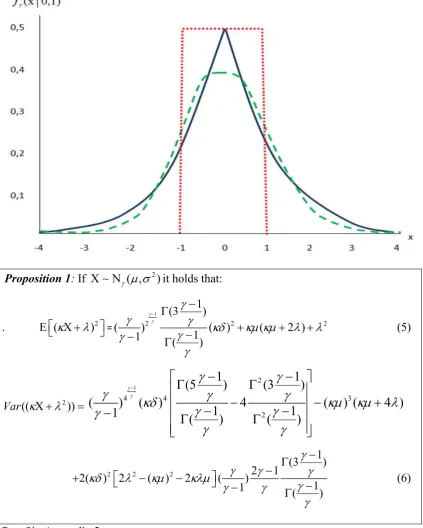
the Uniform but theΝγ( ,σ2).6 Figure 1 clarifies the generalization and represents
the relation between Uniform, Normal and Laplace. This distribution regards a
number of other distributions which are with ‘fat tails’7 and can be used in various
5
See Kitsos and Tavoularis (2009), Kitsos et al. (2012), Halkos and Kitsou(2014). 6
See appendix 1.
7
11
economic analyses like for instance in stock markets. So, the following results are
[image:12.595.88.512.194.723.2]proposed for the form (κg+λ)2 and f xγ( ; , )Σ letting X represent a random variable describing innovation.
Figure 1: Graphical presentation of the relationship between Uniform, Normal and Laplace
: If Χ Ν∼ γ( ,σ2)it holds that:
. Ε(κΧ +λ)2=
1
2 2 2
1
(3 )
( ) ( ) ( 2 )
1
1 ( )
γ γ
γ
γ γ κδ κ κ λ λ
γ γ
γ
− Γ −
+ + +
−
− Γ (5)
2
(( ))
Var κΧ +λ =
1
2
4 4 3
2
1 1
(5 ) (3 )
( ) ( ) 4 ( ) ( 4 )
1 1
1 ( ) ( )
γ γ
γ
γ
γ
κδ
γ
γ
κ
κ
λ
γ
γ
γ
γ
γ
−
− −
Γ Γ
− − +
− −
− Γ Γ
2 2 2
1
(3 )
2 1
2( ) 2 ( ) 2 ( )
1
1 ( )
γ
γ γ γ
κδ λ κ κλ
γ
γ γ
γ
− Γ −
+ − −
−
− Γ (6)
12
With different values of κ and λ a number of calculations for the corresponding TPC can be obtained. Next we present a number of examples.
: Let us assume that TPC = (1/ 4 3 / 8 )− X 2. Then it holds:
1 1 2 1 4 ˆ 1 1 ;
E[T ] 9( ) (3 )
( ) t PC γ γ γ γ γ γ γ γ γ δ − − − − Γ Γ = + ℓ (7)
(
)
4 1 1 2 1 2 1 12
ˆ; 1 1 2 1 1
4 27
1
4 1 4
(5 ) (3 ) (3 )
(6 ) 4 13
( ) ( ) ( )
Var TPCt ( ) 954 ( )
γ γ γ γ γ
γ γ γ
γ γ γ γ
γ γ
γ γ γ γ
γ γ γ
δ δ
− − − − −
− − − − −
Γ Γ Γ
− + +
Γ Γ Γ
=
ℓ
(8)
Based on Example 1, for this particular TPC, it holds that the expected value and variance of TPC can be evaluated for the Uniform, Normal and Laplace distributions as: ; 1 4 1 4 ˆ 1 4 3 ,
E[T ] 9
18
, 1,
, , 2,
, , , t Uniform Normal Laplace PC γ δ γ δ γ δ γ = = = ± + + ∞ = + ℓ (9)
(
)
2 11 45 27 4 27 4 2 7 4 ; 2 ˆ 213 318 (36 )
Var 954 (18
1908 2
, 1,
13 ) , 2,
13 (6 ) , ,
t Uniform Normal Laplac TPC e γ
δ δ γ
δ δ γ
δ δ γ
− = − + = + + + == ±∞ ℓ (10)
: From (9) it obviously holds that the quantity ,
l
t
TPC γ
Ε in the case of Uniform distribution is less than the corresponding Normal distribution, which is less that the corresponding Laplace distribution. That is:
,1 ,2 ,
l l l
t t t
TPC TPC TPC ±∞
Ε < Ε < Ε
For (10) and for 0< <δ 49.074 it holds that:8
13 Figure 2 shows that with γ=1 (the case of uniform) the expected value is less than in the case of γ=2 (the case of normal) and flatter compared to the other two cases. Similarly the results for the comparison between γ=2 (Normal) and γ=±∞ (the case of Laplace) show that Laplace is sharper among them. This implies that changing D the expected value of TPC in the case of the uniform distribution is more stable compared to the other cases. With Laplace being the most sensitive in changing parameter δ, a small change in δ causes a sharp change in the expected value.
Figure 2: Graphical presentations of E[TPCtℓ;γ]=E 2
(1/ 4 3 / 8 )− X withX ~ ( , 2)
γ γ δ
as function of the scale parameterδ , for different values of the parameter γ (blue is for
1
γ ≥ while red is forγ <0).
5. Discussion and policy implications
Environmental taxes should be targeted to the pollutants and should be related
to the environmental damage caused. Without any government intervention countries
(firms) will not take into consideration any environmental damage caused as this may
be either spread across different regions or countries (as in the case of transfrontier
14
one location may play an important role in global climatic changes. The way to cope
with the problem is to tax directly the environmental damage costs due to the damages
imposed.
Specifically, in this research we have considered a general distribution that the
random variable X of the new technologies adopted by a firm, and therefore the total
pollution cost (TPC) follows it covering 3 different lines of thought: a uniform
approach of pollution around the center of pollution, adopting the new technologies; a
normal that is most of the pollution around the centre; and a ‘sharp’ portion of
pollution around the centre, i.e. the Laplace distribution.
Due to this general distribution a weighted location differential tax was
introduced. The proposed tax is differentiated according to the “level of distance”
from the centre of pollution i.e. how far from it has the area being contaminated due
to this particular source of pollution. As a conclusion it is very clear that we are
depending on the assumption of the distribution for the (stochastic) TPC variable.
In this paper as shown the application of the γ)ordered generalized Normal
provides to the researcher the option to choose among three distributions: The
Uniform, Normal and Laplace. That is among no)tails, normal tails, and fat tails. The
decision is also based on the value of δ we choose at the first step – ‘how far’ from the
‘origin of pollution’ we go.
The question of what is the shape of the distribution to be followed is
important. That is why the expected value of the total pollution cost, E(TPC), can be
related to the appropriately calculated variance, Var(TPC), so that approximate .95
confidence interval of the form Ε(TSC) 2± Var TPC( ) to be evaluated, while for a
.99 approximate confidence interval the factor 2 is replaced by 3. As the TPC includes
15
higher taxation under the weighted location tax while the larger the variance the larger
the area polluted and affected socially. Therefore the taxation system should take into
consideration these issues.
Due to difficulties in having available reliable direct cost estimates this
approach may be used with various sensitivity scenarios and existing sensitivity maps
of ecosystems applied to various indirect effects of depositions (see for instance
Kämäri et al., 1992). It is feasible for every country to estimate the area in a number
of sensitivity classes with values determined by ecological criteria like geology,
vegetation, soil type, rainfall amounts etc. For instance acidic depositions vary
significantly with time and location.
If the relationship between source and receptor locations is not considered
then the externality imposed will not be taken into examination. The externality is
considered by the appropriate consideration of the transfer coefficients as provided by
the co)operative programme for monitoring and evaluation of the long range
transmission of air pollutants in Europe (European Monitoring and Evaluation
Program, EMEP). Then mathematical models may be used by policy makers to define
the optimal necessary emissions reductions for each pollution source (country) i and
under the ecosystem sensitivity thresholds (see among others Halkos, 1994).
Acknowledgments
16
References
Böhringer C. and Rutherford T.F. (2002). In Search of a Rationale for Differentiated Environmental Taxes. Centre for European Economic Research (ZEW), Mannheim Discussion Paper No. 02)30. Accessible at: ftp://ftp.zew.de/pub/zew) docs/dp/ dp0230. pdf
Bovenberg, A.L. and F. van der Ploeg (1994), Environmental Policy, Public Finance and the Labor Market in a Second)Best World. Journal of Public Economics,
55, 340)390.
Bovenberg, A.L. and L.H. Goulder (1996), Optimal Environmental Taxation in the Presence of Other Taxes: General Equilibrium Analyses. American Economic Review, 86(4), 985)1000.
Fowlie M. and Muller N. (2013). Market)based emissions regulation when damages vary across sources: What are the gains from differentiation? NBER Working Paper 18801 Accessible at: http://nature.berkeley.edu/~fowlie/Fowlie_Muller_ submit.pdf
Goulder, L. H. (1995), Environmental Taxation and the Double Dividend: A Readers' Guide. International Tax and Public Finance, 2, 157)183.
Goulder, L., I.W.H. Parry and D. Burtraw (1997), Revenue)Raising vs. Other Approaches to Environmental Protection: The Critical Significance of Pre) existing Tax Distortions. RAND Journal of Economics, 28(4), 708)731.
Halkos G.E. (1993). Sulphur abatement policy: implications of cost differentials.
Energy Policy21(10), 1035)1043.
Halkos G.E. (1994). Optimal abatement of sulphur emissions in Europe.
Environmental and Resource Economics, 4(2), 127)150.
Halkos G.E. and Kitsos C. (2005). Optimal pollution level: a theoretical identification,
Applied Economics,37(13), 1475)1483.
Halkos G.E. (1996). Incomplete information in the acid rain game, Empirica,23(2), 129)148.
Halkos G.E. and Kitsou D.C. (2014). Uncertainty in optimal pollution levels: modelling and evaluating the benefit area. Forthcoming in Journal of Environmental Planning and Management 10.1080/09640568.2014.881333
Hutton J.P. and Halkos G.E. (1995). Optimal acid rain abatement policy for Europe: An analysis for the year 2000. Energy Economics, 17(4), 259)275.
17
Kim J.C. and Chang K.B. (1993). An optimal tax/subsidy for output and pollution control under asymmetric information in oligopoly markets. Journal of Regulatory Economics, 5, 193)197.
Kitsos P.C. and Tavoularis K.N. (2009). Logarithmic Sobolev inequalities for information measures, IEEE Transactions of Information Theory, 55(6), 2554) 2561.
Kitsos P.C. and Toulias L.T. (2010). New information measures for the generalized normal distribution. Information, 1, 13)27.
Kitsos P.C., Toulias L.T. and Trandafir P.C. (2012). On the multivariate γ)ordered normal distribution. Far East Journal of Theoretical Statistics, 38(1), 49)73.
McKitrick R. (1999). A Cournot mechanism for pollution control under asymmetric information. Environmental and Resource Economics, 14, 353)363.
Mendelsohn, R. (1986). Regulating heterogeneous emissions. Journal of Environmental Economics and Management, 13 (4), 301.312.
Oates W.E. (1995). Green Taxes: Can We Protect the Environmental and Improve the Tax System at the Same Time. Southern Economic Journal, 61(4), 915)922.
Perman R., Ma Y. and McGilvray J. (2003). Natural Resource and Environmental Economics, 3rd Edition, Longman.
Requate T. (2005). Timing and Commitment of Environmental Policy, Adoption of New Technology, and Repercussions on R&D. Environmental and Resource Economics, 31(2), 175)199.
Terkla, D. (1984), The Efficiency Value of Effluent Tax Revenues. Journal of Environmental Economics and Management, 11, 107)123.
18
Appendix 1
The γ4ordered Normal Distribution
We remind that the normal distribution 2
( ,σ )
Ν , with mean c and varianceσ2
, is defined as:
2
1 2
2
1 1
( ) exp ( )
2 (2 )
f x χ
σ π σ = − − (i)
The multivariate generalization for a multivariate random variable with p)conditions, c mean and matrix covariance Σ is compared with (i) resulting to:
1
1 2 2
1 1
( ) exp ( ) ( )
2 (2 )
p
ϕ χ χ χ
π
Τ −
= − − Σ −
Σ
(ii)
We denote this with Np( , )Σ , Σ =det(Σ).
A more general form of the multivariate distribution was investigated with an extra shape parameter. Indeed Kitsos and Tavoularis (2009) introduced through Logarithm Sobolev Inequalities (LSI) a new family of univariate γ)ordered Normal distribution theΝργ( , )Σ , which generalizes the Normal DistributionΝρ( , )Σ , through an additional parameterγ∈ −ℝ
[ ]
0,1 . The new generalized Normal distribution commonly referred as γ-ordered Normal distribution.When f x( )is the probability density function of a random variable ( , )
ρ γ
Χ Ν∼ Σ then, compared with (ii) above, f x( )is defined as:
[
]
1
2( 1)
2 1
( ; ) p det exp ( )
f x C Q x
γ γ γ γ γ γ − − −
Σ = Σ −
with x
ρ
∈ℝ (iii)
Where Q x( )=(x− )Σ−1(x− )Τas in (ii) with the normality factor
1 2
( 1)
1
2 ( )
1 ( 1) p p p p C p γ γ γ γ π γ γ γ −
− Γ + −
= −
Γ +
(iv)
Where if we set γ=2, i.e. Ν2ρ( , )Σ it follows that:
2 2
( 1) 1 2 ( )
2 ( 1) 2 p p p p C p
π− Γ +
=
Γ +
= 2
2 1 (2 ) 2 p p π π − = (v)
It holds that the multivariate γ)ordered Normal distribution Νγρ( , )Σ for order values of γ=1,2±∞ coincides with
( , )
ρ γ
Ν Σ =
( ) ( , ) ( , ) ( , ) D U L ρ ρ ρ ρ Σ Ν Σ Σ 0 1 2 γ γ γ γ = = = = ±∞ 1, 2
p Dirac distribution
Uniform distibution
Normal distibution
Laplace distibution
=
19
Appendix 2 Proof of Proposition 1
We have seen that:
(
)
2 2 2 2 2 2 2
E[(κX +λ) ]=κ E[X ] 2+ κλE[ ]X +λ =κ Var( )X +E [ ]X +2κλE[ ]X +λ , Assuming X ~ γ( ,δ2) and using the variance of the γ )order Normal distribution,
(see Kitsos and Toulias, 2010) we have that
(
)
2 2 2 2
E[(κX +λ) ]=κ Var( )X + +2κλ +λ . (7) For the variance of Y =(κX +λ)2 we have
2 2 2
4 3 2 3 4 2
4 2 2 2 3 4 2
4 2
4 3 2 2
2
Var( ) E[ ] E [ ] E[( ) ] E [( ) ]
E[ ] 4 λE[ ] 6( ) E[ ] 4 E[ ] E [( ) ]
Kurt( )Var ( ) 6( ) Var( ) 6( ) 4 E [( ) ]
Y Y Y X X
X X X X X
X X X X
κ λ κ λ
κ κ κλ κλ λ κ λ
κ κλ κλ κλ λ κ λ
= − = + − + =
= + + + + − + =
= + + + + − +
As E[X3]=0 ( ( , 2)
γ δ is symmetric distribution i.e. has zero obliquity), thus
eventually, the above equation can be written sequentially as
(
)
(
)
(
)
(
)
4 2 2 2 3 4
2
2 2
4 2 2 2 3 4
2
2 2
3 2 2 2
2
4
3
4
4
Var( ) Kurt( )Var ( ) 6( ) Var( ) 6( ) 4
Var( ) 2
Kurt( )Var ( ) 6( ) Var( ) 6( ) 4
Var( ) 4(
4 Var( ) 2( ) Var( ) 4
Kurt( )Va
)
Y X X X
X
X X X
X
X X
X
κ κλ κλ κλ λ
κ κλ λ
κ κλ κλ κλ λ
κ κλ λ
κ λ κλ κλ
κ = + + + + − + + + = = + + + + = = − + − − − + − + −
2 2 2 3 4
4 2 4 4 2 2
3 3 2 3
4
2
r ( ) 6( ) Var( ) 6( ) 4
Var ( ) ( 2 Var( ) 4(
4( 4 Var( ) 2(
)
) Var( ) 2 ) ( ) ) 4 X X X X X X
κλ κλ κλ λ
κ κ κ κλ λ
κ λ κ λ κλ κλ κλ
+ + + +
− − − − −
− − − − −
And so
4 2 2 4 2 3 3
20
Appendix 3
Checking the differences in variances
Evaluating the differences between the variances of Uniform, Normal and Laplace distributions we may see which are positive or negative, so that to rearrange the order among them.
(A) Between Uniform and Normal (take the difference from (10))
2
12.96 636 0
0
(12.96 636) 0 636
49.074 12.96 δ δ δ δ δ δ − = ⇔ = − = ⇔ = = 0 0 U−N = >
< 0, 49.074 0 49.074 δ δ δ < > < <
The Normal distribution is greater than the Uniform distribution when δ∈(0, 49.074) Otherwise, whenδ >49.074, the Uniform distribution of TPC is greater than its Normal distribution.
( ) ( )
0 49.074
U N
Var TPC Var TPC
δ
< < <
(B) Between Laplace and Normal (take the difference from (10))
2
954 396 0
0
(396 954) 0 954
2.40 396 δ δ δ δ δ δ − − = = + = ⇔ = − = − 0 0 N− = L <
>
( 2.40, 0)
2.40
δ δ
∈ −
< − or δ >0
Because δ is taken always positive, we are interested in the case where δ>0, so the Normal distribution is grater that the Laplace distribution.
( ) ( )
N L
Var TPC <Var TPC
(C) Between Uniform and Laplace (take the difference from (10))
2 1590 383.04
0 (383.04 1590) 1590
4.15 383.04 δ δ δ δ δ δ − − = = − + ⇔ = − = − 0 0 U− = L >
<
( 4.15, 0)
4.15
δ δ
∈ −
< − or δ >0
So, for δ>0, the PSC Uniform distribution is less than the Laplace distribution.
( ) ( )
U L
Var TPC <Var TPC
![Figure 2: Graphical presentations of as function of the scale parameterE[TPC;]tγ =ℓE(1/ 4−3/ 8X)2 withX~(,2γ�γ � δ) δ , for different values of the parameter γ (blue is for γ ≥ while red is for1γ < )](https://thumb-us.123doks.com/thumbv2/123dok_us/1585801.704860/14.595.98.490.239.493/figure-graphical-presentations-function-parametere-different-values-parameter.webp)