Ontology based Distinction between Polysemy and Homonymy

Ontology-based Distinction between Polysemy and Homonymy

Jason Utt

Institut f¨ur Maschinelle Sprachverarbeitung Universit¨at Stuttgart

uttjn@ims.uni-stuttgart.de

Sebastian Pad´o

Seminar f¨ur Computerlinguistik Universit¨at Heidelberg

pado@cl.uni-heidelberg.de

Abstract

We consider the problem of distinguishing polysemous from homonymous nouns. This distinction is often taken for granted, but is seldom operationalized in the shape of an empirical model. We present a first step towards such a model, based on WordNet augmented with ontological classes provided by CoreLex. This model provides apolysemy indexfor each noun which (a), accurately distinguishes between polysemy and homonymy; (b), supports the analysis that polysemy can be grounded in the frequency of the meaning shifts shown by nouns; and (c), improves a regression model that predicts when the “one-sense-per-discourse” hypothesis fails.

1

Introduction

Linguistic studies of word meaning generally divide ambiguity into homonymy and polysemy.

Homony-mous words exhibit idiosyncratic variation, with essentially unrelated senses, e.g.bankas FINANCIAL

INSTITUTION versus as NATURAL OBJECT. In polysemy, meanwhile, sense variation is systematic, i.e., appears for whole sets of words. E.g.,lamb,chickenandsalmonhave ANIMALand FOODsenses.

It is exactly this systematicity that represents a challenge for lexical semantics. While homonymy is assumed to be encoded in the lexicon for each lemma, there is a substantial body of work on dealing with general polysemy patterns (cf. Nunberg and Zaenen (1992); Copestake and Briscoe (1995); Pustejovsky

(1995); Nunberg (1995)). This work is predominantly theoretical in nature. Examples of questions

addressed are the conditions under which polysemy arises, the representation of polysemy in the semantic lexicon, disambiguation mechanisms in the syntax-semantics interface, and subcategories of polysemy.

The distinction between polysemy and homonymy also has important potential ramifications for

computational linguistics, in particular for Word Sense Disambiguation (WSD). Notably, Ide and Wilks

(2006) argue that WSD should focus on modeling homonymous sense distinctions, which are easy to make and provide most benefit. Another case in point is theone-sense-per-discourse hypothesis(Gale

et al., 1992), which claims that within a discourse, instances of a word will strongly tend towards realizing the same sense. This hypothesis seems to apply primarily to homonyms, as pointed out by Krovetz (1998).

Unfortunately, the distinction between polysemy and homonymy is still very much an unsolved question. The discussion in the theoretical literature focuses mostly on clear-cut examples and avoids the broader issue. Work on WSD, and in computational linguistics more generally, almost exclusively

builds on the WordNet (Fellbaum, 1998) word sense inventory, which lists an unstructured set of senses

for each word and does not indicate in which way these senses are semantically related. Diachronic

linguistics proposes etymological criteria; however, these are neither undisputed nor easy to operationalize.

Consequently, there are currently no broad-coverage lexicons that indicate the polysemy status of words,

nor even, to our knowledge, precise, automatizable criteria.

Our goal in this paper is to take a first step towards an automatic polysemy classification. Our approach

is based on the aforementioned intuition that meaning variation is systematic in polysemy, but not in

homonymy. This approach is described in Section 2. We assess systematicity by mapping WordNet senses

OBJECT}above) across the lexicon. We evaluate this model on two tasks. In Section 3, we apply the

measure to the classification of a set of typical polysemy and homonymy lemmas, mostly drawn from the

literature. In Section 4, we apply it to the one-sense-per-discourse hypothesis and show that polysemous

words tend to violate this hypothesis more than homonyms. Section 5 concludes.

2

Modeling Polysemy

Our goal is to take the first steps towards an empirical model of polysemy, that is, a computational model which makes predictions for – in principle – arbitrary words on the basis of their semantic behavior.

The basis of our approach mirrors the focus of much linguistic work on polysemy, namely the fact

that polysemy issystematic: There is a whole set of words which show the same variation between two

(or more) ontological categories, cf. the “universal grinder” (Copestake and Briscoe, 1995). There are

different ways of grounding this notion of systematicity empirically. An obvious choice would be to use a

corpus. However, this would introduce a number of problems. First, while corpora provide frequency information, the role of frequency with respect to systematicity is unclear: should acceptable but rare senses play a role, or not? We side with the theoretical literature in assuming that they do. Another problem with corpora is the actual observation of sense variation. Few sense-tagged corpora exist, and those that do are typically small. Interpreting context variation in untagged corpora, on the other hand,

corresponds to unsupervised WSD, a serious research problem in itself – see, e.g., Navigli (2009).

We therefore decided to adopt a knowledge-based approach that uses the structure of the WordNet

ontology to calculate how systematically the senses of a word vary. The resulting model sets all senses of

a word on equal footing. It is thus vulnerable to shortcomings in the architecture of WordNet, but this

danger is alleviated in practice by our use of a “coarsened” version of WordNet (see below).

2.1 WordNet, CoreLex and Basic Types

WordNet provides only a flat list of senses for each word. This list does not indicate the nature of the sense variation among the senses. However, building on the generative lexicon theory by Pustejovsky (1995), Buitelaar (1998) has developed the “CoreLex” resource. It defines a set of 39 so-calledbasic

typeswhich correspond to coarse-grained ontological categories. Each basic type is linked to one or more WordNetanchor nodes, which define a complete mapping between WordNet synsets and basic types by dominance.1 Table 1 shows the set of basic types and their main anchors; Table 2 shows example lemmas for some basic types.

Ambiguous lemmas are often associated with two or more basic types. CoreLex therefore further

assigns each lemma to what Buitelaar calls apolysemy class, the set of all basic types its synsets belong to; a class with multiple representatives is consideredsystematic. These classes subsume both idiosyncratic and systematic patterns, and thus, despite their name, provide no clue about the nature of the ambiguity. CoreLex makes it possible to represent the meaning of a lemma not through a set of synsets, but instead in terms of a set of basic types. This constitutes an important step forward. Our working hypothesis is that

these basic types approximate the ontological categories that are used in the literature on polysemy to

define polysemy patterns. That is, we can define a meaning shift to mean that a lemma possesses one sense in one basic type, while another sense belongs to another basic type. Naturally, this correspondence is not

perfect: systematic polysemy did not play a role in the design of the WordNet ontology. Nevertheless,

there is a fairly good approximation that allows us to recover many prominent polysemy patterns. Table 3 shows three polysemy patterns characterized in terms of basic types. The first class was already mentioned

before. The second class contains a subset of “transparent nouns” which can denote a container or a

quantity. The last class contains words which describe a place or a group of people.

1_{Note that not all of CoreLex anchor nodes are disjoint; therefore a given WordNet synset may be dominated by two CoreLex}

BT WordNet anchor BT WordNet anchor BT WordNet anchor

abs ABSTRACTION loc LOCATION pho PHYSICALOBJECT

act ACTION log GEOGRAPHICALAREA plt PLANT

agt AGENT mea MEASURE pos POSSESSION

anm ANIMAL mic MICROORGANISM pro PROCESS

art ARTIFACT nat NATURALOBJECT prt PART

atr ATTRIBUTE phm PHENOMENON psy PSYCHOLOGICALFEATURE

cel CELL frm FORM qud DEFINITEQUANTITY

chm CHEMICALELEMENT grb BIOLOGICALGROUP qui INDEFINITEQUANTITY

com COMMUNICATION grp GROUP rel RELATION

con CONSEQUENCE grs SOCIALGROUP spc SPACE

ent ENTITY hum PERSON sta STATE

evt EVENT lfr LIVINGTHING sub SUBSTANCE

fod FOOD lme LINEARMEASURE tme TIME

Table 1: The 39 CoreLex basic types (BTs) and their WordNet anchor nodes

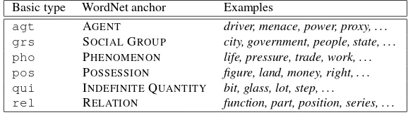
Basic type WordNet anchor Examples

agt AGENT driver, menace, power, proxy, . . . grs SOCIALGROUP city, government, people, state, . . . pho PHENOMENON life, pressure, trade, work, . . . pos POSSESSION figure, land, money, right, . . . qui INDEFINITEQUANTITY bit, glass, lot, step, . . .

rel RELATION function, part, position, series, . . .

Table 2: Basic types with example words

Pattern (Basic types) Examples

ANIMAL, FOOD fowl, hare, lobster, octopus, snail, . . .

ARTIFACT, INDEFINITEQUANTITY bottle, jug, keg, spoon, tub, . . .

ARTIFACT, SOCIALGROUP academy, embassy, headquarters, . . .

Table 3: Examples of polysemous meaning variation patterns

2.2 Polysemy as Systematicity

Given the intuitions developed in the previous section, we define abasic ambiguity as a pair of basic

types, both of which are associated with a given lemma. Thevariation spectrumof a word is then the set

of all its basic ambiguities. For example,bottlewould have the variation spectrum{{art qui} }(cf.

Table 3); the wordcoursewith the three basic typesact,art,grswould have the variation spectrum

{{act art};{act grs};{art grs} }.

There are 39 basic types and thus39·38/2 = 741possible basic ambiguities. In practice, only 663

basic ambiguities are attested in WordNet. We can quantify each basic ambiguity by the number of words that exhibit it. For the moment, we simply interpret frequency as systematicity.2 Thus, we interpret the high-frequency (systematic) basic ambiguities as polysemous, and low-frequency (idiosyncratic) basic

ambiguities as homonymous. Table 4 shows the most frequent basic ambiguities, all of which apply to several hundred lemmas and can safely be interpreted as polysemous. At the other end, 56 of the 663

basic ambiguities are singletons, i.e. are attested by only a single lemma.

In a second step, we extend this classification from basic ambiguities to lemmas. The intuition is again fairly straightforward: A word whose basic ambiguities are systematic will be perceived as polysemous, and as homonymous otherwise. This is clearly an oversimplification, both practically, since we depend

on WordNet/CoreLex having made the correct design decisions in defining the ontology and the basic

types; as well as conceptually, since not all polysemy patterns will presumably show the same degree of systematicity. Nevertheless, we believe that basic types provide an informative level of abstraction, and that our model is in principle even able to account for conventionalized metaphor, to the extent that the corresponding senses are encoded in WordNet.

2

Basic ambiguity Examples

{act com} construction, consultation, draft, estimation, refusal, . . . {act art} press, review, staging, tackle, . . .

{com hum} egyptian, esquimau, kazakh, mojave, thai, . . .

{act sta} domination, excitement, failure, marriage, matrimony, . . . {art hum} dip, driver, mouth, pawn, watch, wing, . . .

Table 4: Top five basic ambiguities with example lemmas

Noun Basic types Noun Basic types

chicken anm fod evt hum lamb anm fod hum salmon anm fod atr nat duck anm fod art qud

Table 5: Words exhibiting the “grinding” (animal – food) pattern

The exact manner in which the systematicity of the individual basic ambiguities of one lemma are combined is not a priori clear. We have chosen the following method. LetP be a basic ambiguity,P(w) the variation spectrum of a lemmaw, andfreq(P)the number of WordNet lemmas with basic ambiguityP. We define the set ofpolysemous basic ambiguitiesPN as theN-most frequent bins of basic ambiguities: PN = {[P1], ...,[P_N]},where[P_i] = {P_j|freq(P_i) = freq(P_j)}andfreq(P_k) > freq(P_l)fork < l.

We call non-polysemous basic ambiguitiesidiosyncratic. Thepolysemy index of a lemmaw,πN(w),is:

πN(w) =

| PN∩ P(w)|

| P(w)| (1)

πN simply measures the ratio ofw’s basic ambiguities which are polysemous, i.e., high-frequency basic ambiguities. πN ranges between 0 and 1, and can be interpreted analogously to the intuition that we have developed on the level of basic ambiguities: high values ofπ(close to 1) mean that the majority of a lemma’s basic ambiguities are polysemous, and therefore the lemma is perceived as polysemous. In contrast, low values of π (close to 0) mean that the lemma’s basic ambiguities are predominantly

idiosyncratic, and thus the lemma counts as homonymous. Again, note that we consider basic ambiguities at the type level, and that corpus frequency does not enter into the model.

This model of polysemy relies crucially on the distinction between systematic and idiosyncratic basic

ambiguities, and therefore in turn on the parameterN.N corresponds to the sharp cutoff that our model

assumes. At theN-th most frequent basic ambiguity, polysemy turns into homonymy. Since frequency

is our only criterion, we have to lump together all basic ambiguities with the same frequency into 135 bins. If we setN = 0, none of the bins count as polysemous, soπ0(w) = 0for allw– all lemmas are homonymous. In the other extreme, we can setN to135, the total number of frequency bins, which

makes all basic ambiguities polysemous, and thus all lemmas:π135(w) = 1for allw. The optimization

ofN will be discussed in Section 3.

2.3 Gradience between Homonymy and Polysemy

We assign each lemma a polysemy index between 0 and 1. We thus abandon the dichotomy that is usually

made in the literature between two distinct categories of polysemy and homonymy. Instead, we consider

polysemy and homonymy the two end points on a gradient, where words in the middle show elements of

both. This type of behavior can be seen even for prototypical examples of either category, such as the

homonymbank, which shows a variation between SOCIALGROUPand ARTIFACT:

(1) a. The bill would forcebanks[...] to report such property. (grs) b. The coinbankwas empty. (art)

Note that this is the same basic ambiguity that is often cited as a typical example of polysemous sense

variation, for example for words likenewspaper.

Homonymous nouns ball, bank, board, chapter, china, degree, fall, fame, plane, plant, pole, post, present, rest,

score, sentence, spring, staff, stage, table, term, tie, tip, tongue

Polysemous nouns bottle, chicken, church, classification, construction, cup, development, fish, glass,

improve-ment, increase, instruction, judgimprove-ment, lamb, manageimprove-ment, newspaper, painting, paper, picture, pool, school, state, story, university

Table 6: Experimental items for the two classeshomandpoly

(anm) andFOOD(fod), a popular example of a regular and productive sense extension. Yet each of the nouns exhibits additional basic types. The nounchickenalso has the highly idiosyncratic meaning of a

person who lacks confidence. Alambcan mean a gullible person,salmonis the name of a color and a

river, and aducka score in the game of cricket. There is thus an obvious unsystematic variety in the words’ sense variations – a single word can show both homonymic as well as polysemous sense alternation.

3

Evaluating the Polysemy Model

To identify an optimal cutoff valueN for our polysemy index, we use a simple supervised approach: we optimize the quality with which our polysemy index models a small, manually created dataset. More specifically, we created a two-class, 48-word dataset with 24 homonymous nouns (classhom) and 24

polysemous nouns (classpoly) drawn from the literature. The dataset is shown in Table 6.

We now rank these items according toπN for different values ofN and observe the ability ofπN

to distinguish the two classes. We measure this ability with the Mann-WhitneyU test, a nonparametric

counterpart of thet-test.3 _{In our case, theU statistic is defined as}

U(N) =

m

X

i=1 n

X

j=1

1(πN(homi)< πN(polyi))

where1is the function function that returns the truth value of its argument (1 for “true”). Informally,

U(N)counts the number of correctly ranked pairs of a homonymous and a polysemous noun.

The maximum forUis the number of item pairs from the classes (24·24 = 576). A score ofU = 576 would mean that everyπN-value of a homonym is smaller than every polysemous value.U = 0means that there are no homonyms with smallerπ-scores. SoU can be directly interpreted as the quality of separation between the two classes. The null hypothesis of this test is that the ranking is essentially

random, i.e., half the rankings are correct4. We can reject the null hypothesis ifU is significantly larger.

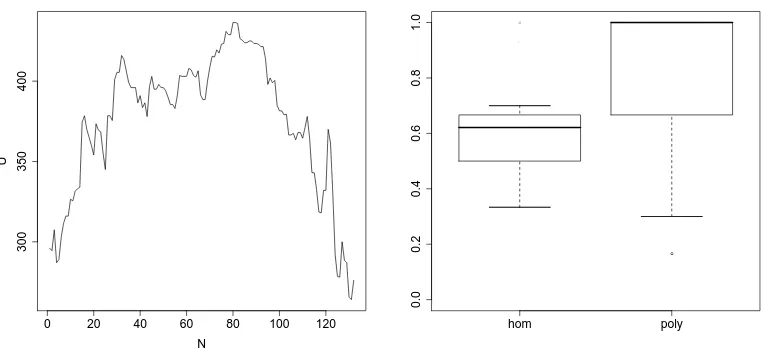
Figure 1(a) shows theU-statistic for all values ofN (between 0 and 135). The left end shows the

quality of separation (i.e. U) for few basic ambiguities (i.e. smallN) which is very small. As soon as we

start considering the most frequent basic ambiguities as systematic and thus as evidence for polysemy,

homandpolybecome much more distinct. We see a clear global maximum ofUforN = 81(U = 436.5). ThisU value is highly significant atp <0.005, which means that even on our fairly small dataset, we can reject the null hypothesis that the ranking is random. π81indeed separates the classes with high confidence:

436.5 of 576 or roughly 75% of all pairwise rankings in the dataset are correct. ForN >81, performance degrades again: apparently these settings include too many basic ambiguities in the “systematic” category, and homonymous words start to be misclassified as polysemous.

The separation between the two classes is visualized in the box-and-whiskers plot in Figure 1(b). We

find that more than 75% of the polysemous words haveπ81> .6. The median value forpolyis 1, thus

for more than half of the classπ81= 1, which can be seen in Figure 2(b) as well. This is a very positive

result, since our hope is that highly polysemous words get high scores. Figure 2(a) shows that homonyms are concentrated in the mid-range while exhibiting a small number ofπ81-values at both extremes.

We take the fact that there is indeed anN which clearly maximizesU as a very positive result that

validates our choice of introducing a sharp cutoff between polysemous and idiosyncratic basic ambiguities.

3

0 20 40 60 80 100 120 300 350 400 N U

(a) TheU_{statistic for different values of the cutoff}N

● ● ● ● ● ● hom poly 0.0 0.2 0.4 0.6 0.8 1.0

(b) Distribution ofπ81values by class

Figure 1: Separation of thehomandpolyclasses in our dataset

These 81 frequency bins contain roughly 20% of the most frequent basic ambiguities. This corresponds to the assumption that basic ambiguities are polysemous if they occur with a minimum of about 50 lemmas.

If we look more closely at those polysemous words that obtain low scores (school, glassandcup),

we observe that they also show idiosyncratic variation as discussed in Section 2.3. In the case ofschool, we have the sensesschooltimeof typetmeandgroup of fishof typegrbwhich one would not expect to

alternate regularly withgrsandart, the rest of its variation spectrum. The wordglasshas the unusual

typeagtdue to its use as a slang term for crystal methamphetamine. Finally,cupis unique in that means both an indefinite quantity as well as the definite measurement equal to half a pint. Only 10 other words

have this variation in WordNet, including such words asmillion andbillion, which are often used to

describe an indefinite but large number.

On the other hand, those homonyms that have a high score (e.g.tie, staff andchina) have somewhat unexpected regularities due to obscure senses. Bothtieandstaff are terms used in musical notation. This

leads to basic ambiguities with thecomtype, something that is very common. Finally, the obviously

unrelated senses forchina,Chinaandporcelain, are less idiosyncratic when abstracted to their types,log

andart, respectively. There are 117 words that can mean a location as well as an artifact, (e.g.fireguard, bath, resort, front, . . .) which are clearly polysemous in that the location is where the artifact is located.

In conclusion, those examples which are most grossly miscategorized byπ81 contain unexpected

sense variations, a number of which have been ignored in previous studies.

ball bank board chapter china degree fall game plane plant pole post present rest score sentence spring staff stage table term tie tip tongue 0 1

(a) Classhom

classification

chicken _bottle construction cup development fish glass improvement increase instruction judgment lamb management newspaper painting paper picture pool school state story university church 0 1

(b) Classpoly

4

The One-Sense-Per-Discourse Hypothesis

The second evaluation that we propose for our polysemy index concerns a broader question on word

sense, namely the so-calledone-sense-per-discourse (1spd)hypothesis. This hypothesis was introduced

by Gale et al. (1992) and claims that “[...] if a word such assentence appears two or more times in a well-written discourse, it is extremely likely that they will all share the same sense”. The authors verified their hypothesis on a small experiment with encouraging results (only 4% of discourses broke

the hypothesis). Indeed, if this hypothesis were unreservedly true, then it would represent a very strong

global constraint that could serve to improve word sense disambiguation – and in fact, a follow-up paper

by Yarowsky (1995) exploited the hypothesis for this benefit.

Unfortunately, it seems that1spd does not apply universally. At the time (1992), WordNet had not yet emerged as a widely used sense inventory, and the sense labels used by Gale et al. were fairly coarse-grained ones, motivated by translation pairs (e.g., Englishdutytranslated as Frenchdroit (tax)

vs.devoir (obligation)), which correspond mostly to homonymous sense distinctions.5 Current WSD, in

contrast, uses the much more fine-grained WordNet sense inventory which conflates homonymous and

polysemous sense distinctions. Now,1spdseems intuitively plausible for homonyms, where the senses

describe different entities that are unlikely to occur in the same discourse (or if they do, different words will be used). However, the situation is different for polysemous words: In a discourse about a party,bottle

might felicitously occur both as an object and a measure word. A study by Krovetz (1998) confirmed this intuition on two sense-tagged corpora, where he found 33% of discourses to break1spd. He suggests that knowledge about polysemy classes can be useful as global biases for WSD.

In this section, we analyze the sense-tagged SemCor corpus in terms of the basic type-based framework of polysemy that we have developed in Section 2 both qualitatively and quantitatively to demonstrate that basic types, and our polysemy indexπ, help us better understand the1spdhypothesis.

4.1 Analysis by Basic Types and One-Basic-Type-Per-Discourse

The first step in our analysis looks specifically at the basic types and basic ambiguities we observe in discourses that break1spd. Our study reanalyses SemCor, a subset of the Brown corpus annotated

ex-haustively with WordNet senses (Fellbaum, 1998). SemCor contains a total of 186 discourses, paragraphs

of between 645 and 1023 words. These 186 discourses, in combination with 1088 nouns, give rise to

7520lemma-discourse pairs, that is, cases where a sense-tagged lemma occurs more than once within a

discourse.6 These 7520 lemma-discourse pairs form the basis of our analysis. We started by looking at the relative frequency of1spd. We found that the hypothesis holds for 69% of the lemma-discourse pairs, but not for the remaining 31%. This is a good match with Krovetz’ findings, and indicates that there are many discourses where there lemmas are used in different senses.

In accordance with our approach to modeling meaning variation at the level of basic types, we

implemented a “coarsened” version of1spd, namelyone-basic-type-per-discourse (1btpd). This hypothesis

is parallel to the original, claiming that it is extremely likely that all words in a discourse share the samebasic type. As we have argued before, the basic-type level is a fairly good approximation to the most important ontological categories, while smoothing over some of the most fine-grained (and most

troublesome) sense distinctions in WordNet. In this vein,1btpdshould get rid of “spurious” ambiguity, but preserve meaningful ambiguity, be it homonymous or polysemous. In fact, the basic type with most

of these “within-basic-type” ambiguities is PSYCHOLOGICALFEATURE, which contains many subtle

distinctions such as the following senses ofperception:

a. a way of conceiving something b. the process of perceiving

c. knowledge gained by perceiving d. becoming aware of something via the senses

Such distinctions are collapsed in1btpd. In consequence, we expect a noticeable, but limited, reduction in

5

Note that Gale et al. use the term “polysemy” synonymously with “ambiguous”. 6

Basic ambiguity most common breaking words freq(Pbreaks1btpd) freq(P) N

{com psy} evidence, sense, literature, meaning, style, . . . 89 365 13

{act psy} study, education, pattern, attention, process, . . . 88 588 7

{psy sta} need, feeling, difficulty, hope, fact, . . . 79 338 14

{act atr} role, look, influence, assistance, interest, . . . 79 491 9

{act art} church, way, case, thing, design, . . . 67 753 2

{act sta} operation, interest, trouble, employment, absence, . . . 60 615 4

{act com} thing, art, production, music, literature, . . . 59 755 1

{atr sta} life, level, desire, area, unity, . . . 58 594 6

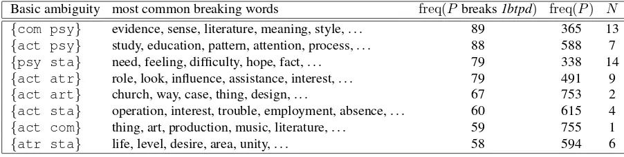
Table 7: Most frequent basic ambiguities that break the1btpdhypothesis in SemCor

the cases that break the hypothesis. Indeed,1btpdholds for 76% of all lemma-discourse pairs, i.e., for 7% more than1spd. For the remainder of this analysis, we will test the1btpdhypothesis instead of1spd.

The basic type level also provides a good basis to analyze the lemma-discourse pairs where the

hypothesis breaks down. Table 7 shows the basic ambiguities that break the hypothesis in SemCor most

often. The WordNet frequencies are high throughout, which means that these basic ambiguities are

poly-semous according to our framework. It is noticeable that the two basic types PSYCHOLOGICAL FEATURE and ACTION participate in almost all of these basic ambiguities. This observation can be explained

straightforwardly through polysemous sense extension as sketched above: Actions are associated, among other things, with attributes, states, and communications, and discussion of an action in a discourse can

fairly effortlessly switch to these other basic types. A very similar situation applies to psychological features, which are also associated with many of the other categories. In sum, we find that the data bears out our hypothesis: almost all of the most frequent cases of several-basic-types-per-discourse clearly

correspond to basic ambiguities that we have classified as polysemous rather than homonymous.

4.2 Analysis by Regression Modeling

This section complements the qualitative analysis of the previous section with a quantitative analysis

which predicts specifically for which lemma-discourse pairs1btpdbreaks down. To do so, we fit a logit mixed effects model (Breslow and Clayton, 1993) to the SemCor data. Logit mixed effects models can

be seen as a generalization of logistic regression models. They explain a binaryresponse variableyin terms of a set offixed effectsx, but also include a set ofrandom effectsx′_{. Fixed effects correspond to} “ordinary” predictors as in traditional logistic regression, while random effects account for correlations in the data introduced by groups (such as items or subjects) without ascribing these random effects the same causal power as fixed effects – see, e.g., Jaeger (2008) for details.

The contribution of each factor is modelled by a coefficientβ, and their sum is interpreted as the

logit-transformed probability of a positive outcome for the response variable:

p(y= 1) = 1

1 +e−z withz=

X βixi+

X β′

jx′j (2)

Model estimation is usually performed using numeric approximations. The coefficientsβ′_{of the random}

effects are drawn from a multivariate normal distribution, centered around 0, which ensures that the

majority of random effects are ascribed very small coefficients.

From a linguistic perspective, a desirable property of regression models is that they describe the importance of the different effects. First of all, each coefficient can be tested for significant difference

to zero, which indicates whether the corresponding effect contributes significantly to modeling the data. Furthermore, the absolute value of eachβican be interpreted as thelog odds– that is, as the (logarithmized)

change in the probability of the response variable being positive depending onxibeing positive.

In our experiment, each datapoint corresponds to one of the 7520 lemma-discourse pair from SemCor

(cf. Section 4.1). The response variable is binary: whether1btpdholds for the lemma-discourse pair or

not. We include in the model five predictors which we expect to affect the response variable: three fixed

Predictor Coefficient Odds (95% confidence interval) Significance

Number of basic types -0.50 0.61 (0.59–0.63) ***

Log length of discourse (words) -0.60 1.83 (1.14–2.93) –

Polysemy index (π81) -0.91 0.40 (0.35–0.46) ***

Table 8: Logit mixed effects model for the response variable “one-basic-type-per-discourse (1btpd) holds” (SemCor; random effects: discourse and lemma; significances: –:p >0.05; ***:p <0.001)

number of its basic types, i.e. the size of its variation spectrum. We expect that the more ambiguous a

noun, the smaller the chance for1btpd. We expect the same effect for the (logarithmized) length of the discourse in words: longer discourses run a higher risk for violating the hypothesis. Our third fixed effect

is the polysemy indexπ81, for which we also expect a negative effect. The two random effects are the

identity of the discourse and the noun. Both of these can influence the outcome, but should not be used as full explanatory variables.

We build the model in the R statistical environment, using thelme47package. The main results are shown in Table 8. We find that the number of basic types has a highly significant negative effect on the

1btpdhypothesis(p <0.001). Each additional basic type lowers the odds for the hypothesis by a factor

ofe−0.50

≈0.61. The confidence interval is small; the effect is very consistent. This was to be expected – it would have been highly suspicious if we had not found this basic frequency effect. Our expectations are not met for the discourse length predictor, though. We expected a negative coefficient, but find a positive one. The size of the confidence interval shows the effect to be insignificant. Thus, we have to assume that

there is no significant relationship between the length of the discourse and the1btpdhypothesis. Note

that this outcome might result from the limited variation of discourse lengths in SemCor: recall that no

discourse contains less than 645 or more than 1023 words.

However, we find a second highly significant negative effect(p <0.001)in our polysemy indexπ81. With a coefficient of -0.91, this means that a word with a polysemy index of 1 is only 40% as likely to preserve1btpd than a word with a polysemy index of 0. The confidence interval is larger than for the number of basic types, but still fairly small. To bolster this finding, we estimated a second mixed effects model which was identical to the first one but did not containπ81as predictor. We tested the

difference between the models with a likelihood ratio test and found that the model that includesπ81is

highly preferred (p <0.0001;D=−2∆LL= 40;df = 1).

These findings establish that our polysemy indexπ can indeed serve a purpose beyond the direct modeling of polysemy vs. homonymy, namely to explain the distribution of word senses in discourse

better than obvious predictors like the overall ambiguity of the word and the length of the discourse can. This further validates the polysemy index as a contribution to the study of the behavior of word senses.

5

Conclusion

In this paper, we have approached the problem of distinguishing empirically two different kinds of word sense ambiguity, namely homonymy and polysemy. To avoid sparse data problems inherent in

corpus work on sense distributions, our framework is based on WordNet, augmented with the ontological

categories provided by the CoreLex lexicon. We first classify the basic ambiguities (i.e., the pairs of

ontological categories) shown by a lemma as either polysemous or homonymous, and then assign the ratio of polysemous basic ambiguities to each word as its polysemy index.

We have evaluated this framework on two tasks. The first was distinguishing polysemous from homonymous lemmas on the basis of their polysemy index, where it gets 76% of all pairwise rankings correct. We also used this task to identify an optimal value for the threshold between polysemous and homonymous basic ambiguities. We located it at around 20% of all basic ambiguities (113 of 663 in the top 81 frequency bins), which apparently corresponds to human intuitions. The second task was an analysis of the one-sense-per-discourse heuristic, which showed that this hypothesis breaks down

frequently in the face of polysemy, and that the polysemy index can be used within a regression model to predict the instances within a discourse where this happens.

It may seem strange that our continuous index assumes a gradient between homonymy and polysemy. Our analyses indicate that on the level of actual examples, the two classes are indeed not separated by a clear boundary: many words contain basic ambiguities of either type. Nevertheless, even in the linguistic

literature, words are often considered as either polysemous or homonymous. Our interpretation of this

contradiction is that some basic types (or some basic ambiguities) are more prominent than others. The

present study has ignored this level, modeling the polysemy index simply on the ratio of polysemous patterns without any weighting. In future work, we will investigate human judgments of polysemy vs.

homonymy more closely, and assess other correlates of these judgments (e.g., corpus counts).

A second area of future work is more practical. The logistic regression incorporating our polysemous index predicts, for each lemma-discourse pair, the probability that the one-sense-per-discourse hypothesis

is violated. We will use this information as a global prior on an “all-words” WSD task, where all occurrences of a word in a discourse need to be disambiguated. Finally, Stokoe (2005) demonstrates the chances for improvement in information retrieval systems if we can reliably distinguish between

homonymous and polysemous senses of a word.

References

Breslow, N. and D. Clayton (1993). Approximate inference in generalized linear mixed models. Journal

of the American Statistical Society 88(421), 9–25.

Buitelaar, P. (1998). CoreLex: An ontology of systematic polysemous classes. InProceedings of FOIS, Amsterdam, Netherlands, pp. 221–235.

Copestake, A. and T. Briscoe (1995). Semi-productive polysemy and sense extension. Journal of

Semantics 12, 15–67.

Fellbaum, C. (1998). WordNet: An Electronic Lexical Database. MIT Press.

Gale, W. A., K. W. Church, and D. Yarowsky (1992). One sense per discourse. InProceedings of HLT,

Harriman, NY, pp. 233–237.

Ide, N. and Y. Wilks (2006). Making sense about sense. In E. Agirre and P. Edmonds (Eds.),Word Sense Disambiguation: Algorithms and Applications, pp. 47–74. Springer.

Jaeger, T. (2008). Categorical data analysis: Away from ANOVAs and toward Logit Mixed Models.

Journal of Memory and Language 59(4), 434–446.

Krovetz, R. (1998). More than one sense per discourse. InProceedings of SENSEVAL, Herstmonceux

Castle, England.

Navigli, R. (2009). Word Sense Disambiguation: a survey. ACM Computing Surveys 41(2), 1–69.

Nunberg, G. (1995). Transfers of meaning. Journal of Semantics 12(2), 109–132.

Nunberg, G. and A. Zaenen (1992). Systematic polysemy in lexicology and lexicography. InProceedings

of Euralex II, Tampere, Finland, pp. 387–395.

Pustejovsky, J. (1995). The Generative Lexicon. Cambridge MA: MIT Press.

Stokoe, C. (2005). Differentiating homonymy and polysemy in information retrieval. InProceedings of

the conference on Human Language Technology and Empirical Methods in NLP, Morristown, NJ, pp.

403–410.