Improving Chinese Word Segmentation by Adopting Self Organized Maps of Character N gram

Improving Chinese Word Segmentation by Adopting

Self-Organized Maps of Character N-gram

Chongyang Zhang iFLYTEK Research

[email protected]

Zhigang Chen iFLYTEK Research  [email protected]

Guoping Hu 

iFLYTEK Research

[email protected]

 

   

Abstract

Character-based tagging method has achieved great success in Chinese Word Segmentation (CWS). This paper proposes a new approach to improve the CWS tagging accuracy by combining Self-Organizing Map (SOM) with structured support vector machine (SVM) for utilization of enormous unlabeled text corpus. First, character N-grams are clustered and mapped into a low-dimensional space by adopting SOM algorithm. Two different maps are built based on the N-gram’s preceding and succeeding context respectively. Then new features are extracted from these maps and integrated into the structured SVM methods for CWS. Experimental results on Bakeoff-2005 database show that SOM-based features can contribute more than 7% relative error reduction, and the structured SVM method for CWS proposed in this paper also outperforms traditional conditional random field (CRF) method.

1

Introduction

It is well known that there is no space or any other separators to indicate the word boundary in Chinese. But word is the basic unit for most of Chinese natural language process tasks, such as Machine Translation, Information Extraction, Text Categorization and so on. As a result, Chinese word segmentation (CWS) becomes one of the most fundamental technologies in Chinese natural language process.

In the last decade, many statistics-based methods for automatic CWS have been

proposed with development of machine learning and statistical method (Huang and Zhao, 2007). Especially, the character-based tagging method which was proposed by Nianwen Xue (2003) achieves great success in the second International Chinese word segmentation Bakeoff in 2005 (Low et al., 2005). The character-based tagging method formulates the CWS problem as a task of predicting a tag for each character in the sentence, i.e. every character is considered as one of four different types in 4-tag set: B (begin of word), M (middle of word), E (end of word), and S (single-character word).

Most of these works train tagging models only on limited labeled training sets, without using any unsupervised learning outcomes from innumerous unlabeled text. But in recent years, researchers begin to exploit the value of enormous unlabeled corpus for CWS. Some statistics information on co-occurrence of sub-sequences in the whole text has been extracted from unlabeled data and been employed as input features for tagging model training (Zhao and Kit , 2007).

Word clustering is a common method to utilize unlabeled corpus in language processing research to enhance the generalization ability, such as part-of-speech clustering and semantic clustering (Lee et al., 1999 and B Wang and H

characters of the word “Turkey” in Chinese), if we could cluster the two bigrams together according to unlabeled corpus and employ it as a feature for supervised training of tagging model, maybe we will know that there should be a word boundary after “耳/其” though we only find the existence of word boundary after “色/列” in the training data. So we investigate how to apply clustering method onto unlabeled data for the purpose of improving CWS accuracy in this paper.

This paper proposes a novel method of using unlabeled data for CWS, which employs Self-Organizing Map (SOM) (Kohonen 1982) to organize Chinese character N-grams on a two-dimensional array, named as “N-gram cluster map” (NGCM), in which the character N-grams similar in grammatical structure and semantic meaning are organized in the same or adjacent position. Two different arrays are built based on the N-gram’s preceding context and succeeding context respectively because sometimes N-gram is just a part of Chinese word and does not share similar preceding and succeeding context in the same time. Then NGCM-based features are extracted and applied to tagging model of CWS. Two tagging models are investigated, which are structured support vector machine (SVM) (Tsochantaridis et al., 2005) model and

Confidential Random Fields (CRF) (Lafferty et al., 2001). The experimental results show that NGCM is really helpful to CWS. In addition, we find that the structured SVM achieves better performance than CRF.

The rest of this paper is organized as follows: Section 2 presents self-organizing map and the idea of N-gram cluster maps. Section 3 describes structured SVM and how to use the NGCMs based features in CWS. Section 4 shows experimental results on Bakeoff-2005 database and Section 5 gives our conclusion.

2

N-gram cluster maps

Supervised learning method for CWS needs enough pre-labeled corpus with word boundary information for training. The final CWS performance relies heavily on the quality of the training data. The training data is limited and cannot cover completely the linguistic phenomenon. But unlabeled corpus can be

obtained easily from internet. One intuitive method is to extract information from unsupervised learning results from enormous unlabeled data to enhance supervised learning.

2.1 Self-Organizing Map

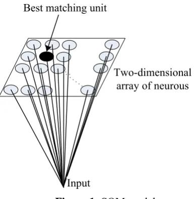
The Self-Organizing Map (SOM) (Kohonen 1982), sometimes called Kohonen map, was developed by Teuvo Kohonen in the early 1980s. Different from other clustering method, SOM is a type of artificial neural network on the basis of competitive learning to visualize higher dimensional data in a low-dimensional space (usually 1D or 2D) while preserving the topological properties of the input space. Figure 1 displays a 2D SOM.

Best matching unit

Input

[image:2.595.307.500.291.489.2]

Two-dimensional array of neurous

Figure 1: SOM model

In SOM, the input is a lot of data samples, and each sample is represented as a vector

,

1,2,...,

i

x i

=

M

, where M is the number of the

input vectors. SOM will cluster all these samples into L neurons, and each neuron is

associated with a weight vector

w i

_i

,

=

1,2,...,

L

, where

L

is the total number of the neurons. 

w

_j 

is  of the same dimensions as the input data vectors

x

_i. The learning algorithm of SOM is as follows:

1. Randomize every neuron’s weight vector

i

w

;

3. Find the winning neuron

j

 

, whose associate weight vector

w

_j has the minimal distance to

x

_t ;

4. Update the weight vector of all the neurons according to the following formula:

( , )( )

i i t i

w ←w +

ηφ

i j x −w

Where

η

_{is the learning-rate and}

φ

( , )

i j

is the neighborhood function. A simple choice defines

φ

( , ) 1

i j

=

_{for all neuron}

i

in a neighborhood of radius r of neuron

j

and

φ

( , ) 0

i j

=

for all other neurons.

η

and

φ

( , )

i j

usually varied dynamically

during learning for best results;

5. Continue step 2 until maximum number of iterations has been reached or no noticeable changes are observed.

2.2 SOM-based N-gram cluster maps

Self-organizing semantic maps (Ritter and Kohonen 1989, 1990) are SOMs that have been organized according to word similarities, measured by the similarity of the short contexts of the words. Our algorithm of building N-gram cluster maps is similar to self-organizing semantic maps. Because sometimes N-gram is just part of Chinese word and do not share similar preceding and succeeding context in the same time, so we build two different maps according to the preceding context and the succeeding context of N-gram individually. In the end we build two NGCMs: NGCMP (NGCM according to preceding context) and NGCMS (NGCM according to succeeding context).

In this paper we only consider bigram cluster maps. So our purpose is to acquire a 2GCMP and a 2GCMS. The large-scale unlabeled corpus

we used for training NGCMs is about 3.5G in size. It was obtained easily from websites like Sohu, Netease, Sina and People Daily. When the cut-off threshold is set to 5, we got about 9K different characters and 380K different bigrams by counting the corpus. For each bigram, a 9K-dimensional sparse vector can be derived from the preceding character of the bigram. Therefore a collection of 380K vector samples are generated, which is denoted as P. Another

vector collection S which considers succeeding

character was obtained using the same method.

Our implementation used SOM-PAK package Version 1.0 (Kohonen et al., 1996). We

set the topology type to rectangular and the map size to15 15× . In the training process, we used

P and S as input data respectively. After the

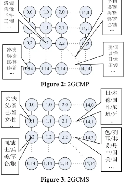
[image:3.595.307.518.257.568.2]

training we acquired a 2GCMP and a 2GCMS, meanwhile each bigram was mapped to one neuron. Because the number of neurons is much smaller than the number of bigrams, each neuron in the map was labeled with multiple bigrams. The 2GCMP and 2GCMS are shown in Figure 2 and Figure 3 respectively. The comment boxes in the figures show some samples of bigrams mapped in the same neuron.

Figure 2: 2GCMP

0,0

0,1 1,1 2,1

0,2 1,2 2,2

1,0 2,0

14,14 14,2 14,0

0,14 1,14 2,14

14,1

色/列 耳/其 苏/丹 中/国 美/国

…

丈/夫 父/亲 已/婚 女/性 …

同/志 士/兵 美/军 台/胞

...

日/本 德/国 印/尼 班/牙

...

Figure 3: 2GCMS

used in the self-organizing semantic maps. We found that the bigrams of “巴/基”, “埃/塞” and “俄/罗” will never be assigned to the same neuron again, which indicates that we need to build two NGCMs according to preceding and succeeding context separately.

3

Integrate NGCM into Structured

SVM for CWS

3.1 Structured support vector machine

The structured support vector machine can learn to predict structured

y

, such as trees sequences or sets, from x based on large-margin approach. We employ a structured SVM that can predict a sequence of labels

( ,...,

1 T

)

y

=

y

y

for a given observation sequence

( ,..., )

1 T

x

=

x

x

, where

t

y

∈

∑ ,∑ is the label set for y.

There are two types of features in the structured SVM: transition features (interactions between neighboring labels along the chain), emission features (interactions between attributes of the observation vectors and a specific label).we can represent the input-output pairs via joint feature map (JFM)

1 1 1 1

( )

( )

( , )

( )

(

)

T

t c t

t T

c t c t

t

x

y

x y

y

y

φ

ψ

η

= − + =

⎛

_{⊗ Λ}

⎞

⎜

⎟

⎜

⎟

=

⎜

⎟

Λ

⊗ Λ

⎜

⎟

⎝

⎠

∑

∑

where

{

1 2 1 2 , 1, 0,

( ) ( ( , ), ( , ),..., (

, ))'

{0,1} , { , ,...,

}

Kronecker delta ,

c K K K i j i j i j

y

y y

y y

y

y

y

y y

y

δ

δ

δ

δ δ

=_≠ ∑

Λ

≡

∈

∈

=

=

( )

x

φ

denotes an arbitrary feature representation of the inputs. The sign " "⊗ expresses tensor

product defined as ⊗ : d k

R

×

R

→

R

dk ,

[

a

⊗

b

]

i+ −_{( 1)}j d

=

[ ] [ ]

a b

i j.

T

is the length of an observation sequence.

η

≥

0

is a scaling factor which balances the two types of contributions.

Note that both transition features and emission features can be extended by including higher-order interdependencies of labels (e.g.

1 2

( )

(

)

(

)

c t c t c t

y

y

+

y

+

Λ

⊗ Λ

⊗ Λ

),by including

input features from a window centered at the

current position (e.g. replacing

( )

t

x

φ

with

(

t r

,..., ,...

t t r

)

x

x

x

φ

− + _{)or by combining}

higher-order output features with input features (e.g.

1

( )

t c

( )

t c

(

t

)

t

φ

x

y

y

+

⊗ Λ

⊗ Λ

∑

)

The w-parametrized discriminant function

:

F X Y× →R interpreted as measuring the

compatibility of x and y is defined as:

( , ; ) , ( , )

F x y w = w

ψ

x y

So we can maximize this function over the response variable to make a prediction

( ) arg max ( , , )

y Y

f x F x y w

∈

=

Training the parameters can be formulated as the following optimization problem.

, ₁

1

min

,

2

. . ,

:

, ( , )

( , )

( , )

n i w i

i i i i i i i

C

w w

n

s t

i

y

Y

w

x y

x y

y y

ξ

ξ

ψ

ψ

ξ

=

+

∀ ∀ ∈

−

≥ Δ

−

∑

where n is the number of the training samples,

i

ξ

is a slack variable , C≥0 is a constant controlling the tradeoff between training error minimization and margin maximization,

1

( , )

y y

Δ

is the loss function ,usually the number of misclassified tags in the sentence.

3.2 Features set for tagging model

For a training sample denoted as

1

( ,..., )

T

x

=

x

x

and

y

=

( ,...,

y

1

y

T

)

. We chose

first-order interdependencies of labels to be transition features, and dependencies between labels and N-grams (n=1, 2, 3) at current position in observed input sequence to be emission features.

So our JFM is the concatenation of the follow vectors 1 1 1

( )

(

)

T

c t c t

t

y

y

−

+

=

Λ

⊗ Λ

∑

,

1

(

)

( ),

{ 1,0,1}

T

t m c t

t

x

y

m

φ

+ =

⊗ Λ

∈ −

∑

1

1

(

,

)

( ),

{ 2, 1,0,1}

T

t m t m c t

t

x

x

y

m

φ

+ + + =

⊗ Λ

∈ − −

∑

1 1

1

(

,

,

)

( ),

{ 1,0,1}

T

t m t m t m c t

t

x

x

x

y

m

φ

+ − + + + =

⊗ Λ

∈ −

∑

emission features of N-grams (n=1, 2) at

y

₃. The emission features of 3-grams are not shown here because of the large number of the interactions.

1

y y₂ y3 y4

1

x x₂ x3 x4

5

y

5

[image:5.595.92.276.128.206.2]

x

Figure 4: the transition features and the

emission features at

y

_{3 for structured SVM}

3.3 Using NGCM in CWS

Two methods can be used for extracting the features from NGCMs to expend features definition in section 3.2.

One method is to treat NGCM just as a clustering tool and do not take into account the similarity between adjacent neurons. So a new feature with L dimensions can be generated,

where L is the number of the neurons or classes.

Only one value of the L dimension equals to 1

and others equal to 0. We call it NGCM

clustering feature.

Another way of using the NGCM is to adopt the position of the neurons which current N-gram mapped in the NGCM as a new feature. So every feature has D dimensions (D equals to

the dimension of the NGCM, every dimension is corresponding to the coordinate value in the NGCM). In this way, N-gram which is originally represented as a high dimensional vector based on its context is mapped into a very low-dimensional space. We call it NGCM

mapping feature.

In this paper, we only consider the NGCM clustering or mapping features related to the current label

y

_i. We also extract features from the quantization error of current N-gram because the result of the NGCM is very noisy. Then our previous JFM in section 3.2 is concatenated with the following features:

2GCMS 1

1

( , ) ( ), { 2, 1}

T

t m t m c t

t

x x y m

ϕ + + +

=

⊗ Λ ∈ − −

∑

2GCMP 1

1

(

,

)

( ),

{0,1}

T

t m t m c t

t

x

x

y

m

ϕ

+ + + =

⊗ Λ

∈

∑

2GCMS 1

1

( , ) ( ), { 2, 1}

T

t m t m c t

t

x x y m

η

+ + +

=

⊗ Λ ∈ − −

∑

2GCMP 1

1

(

)

( ),

{0,1}

T

t m t m c t

t

x

x

y

m

η

+ + + =

⊗ Λ

∈

∑

 

where

ϕ

2GCMS

( )

x

denotes the NGCM feature from 2GCMS,

ϕ

2GCMP

( )

x

denotes the NGCM feature from 2GCMP. 

η

NGCM

( )

x

denotes the quantization error of current N-gram xon its NGCM. 

In 15 15× size NGCM, when we use the

NGCM clustering feature

ϕ

2GCMS

( )

x

and

2GCMP

_{( )}

x

ϕ

_∈

_{0,1}

15 15× _{. When we use the}

NGCM mapping feature

ϕ

2GCMS

( )

x

and

2GCMP

_{( )}

x

ϕ

_∈

_{0,1,...,14}

2

.  Notice that the dimension of the NGCM clustering feature is much higher than the NGCM mapping feature.

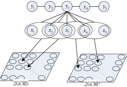
As an example, the process of import features from NGCMs at

y

₃ is presented in Figure 5.

1

y y2 y3 y4

1

x x₂ x3 x4 5

y

5

x

2GCMS 2GCMP

Figure 5: Using 2GCMS and 2GCMP as input

to structured SVM

4

Applications and Experiments

4.1 Corpus

We use the data adopted by the second International Chinese Word Segmentation Bakeoff (Bakeoff-2005). The corpus size information is listed in Table 1.

Corpus As CityU MSRA PKU

Training(M) 5.45 1.46 2.37 1.1

Test(K) 122 41 107 104

Table 1: Corpus size of Bakeoff-2005 in

[image:5.595.308.516.372.514.2]

4.2 Text Preprocessing

Text is usually mixed up with numerical or alphabetic characters in Chinese natural language, such as “我在 office 上班到晚上 9

点”. These numerical or alphabetic characters are barely segmented in CWS. Hence, we treat these symbols as a whole “character” according to the following two preprocessing steps. First replace one alphabetic character to four continuous alphabetic characters with E1 to E4 respectively, five or more alphabetic characters with E5. Then replace one numerical number to four numerical numbers with N1 to N4 and five or more numerical numbers with N5. After text preprocessing, the above examples will be “我 在E5上班到晚上N1点”.

4.3 Character-based tagging method for CWS

Previous works show that 6-tag set achieved

a better CWS performance (Zhao et al.,

2006). Thus, we opt for this tag set. This

6-tag set adds ‘B2’ and ’B3’ to 4-6-tag set

which stand for the type of the second and

the third character in a Chinese word

respectively. For example, the tag sequence

for the sentence “上海世博会/将/持续/半

年

(Shanghai World Expo / will / last / six

months)” will be “B B2 B3 M E S B E B E”.

4.4 Experiments

The F-measure is employed for evaluation, which is defined as follows:

num of correctly segmented words Precision: P

num of the system output words

=

num of correctly segmented words Recall: R

num of total words in test data

=

2 P R

F-measure: F

P R

× ×

=

+

To compare with other discriminative learning methods we first developed a baseline system using conditional random field (CRF) without using NGCM feature and then we developed another CRF system: CFCRF (using NGCM clustering features). In the end we developed three structured SVM CWS systems: SVM (without using NGCM features), CFSVM

(using NGCM clustering features), and MFSVM (using NGCM mapping features). The features for the baseline CRF system are the same with the SVM system. The features for CFCRF are the same with CFSVM. The result of the CRF system using NGCM mapping features cannot be given here, because it is difficult to support continuous-value features for CRF method which is based on the Maximum Entropy Model.

We use CRF++ version 0.5 (Kudu, 2009) to build our CRF models. The cut-off threshold is set to 2(using the features that occurs no less than 2 times in the given training data) and the hyper-parameter is set to 4.5. We use hmm

svm

version 3.1 to build our structured SVM models. The cut-off threshold is set to 2. The precision parameter is set to 0.1. The tradeoff between training error minimization and margin maximization is set to 1000.

The comparisons between CRF, CFCRF, SVM, CFSVM and MFSVM are shown in Table 2.

Corpus As CityU MSRA PKU

CRF baseline

P 0.945 0.943 0.971 0.953 R 0.955 0.942 0.970 0.946 F 0.950 0.942 0.971 0.950

CFCRF

P 0.948 0.956 0.973 0.959 R 0.959 0.961 0.972 0.952 F 0.953 0.958 0.973 0.955

SVM P 0.949 0.957 0.972 0.953

R 0.959 0.959 0.972 0.946 F 0.954 0.958 0.972 0.950

CFSVM

P 0.952 0.959 0.974 0.958 R 0.960 0.964 0.974 0.952 F 0.956 0.961 0.974 0.955

MFSVM

P 0.950 0.957 0.974 0.958 R 0.961 0.963 0.974 0.951 F 0.956 0.960 0.974 0.954 Table 2: The results of our systems

4.5 Discussion

From Table 2, we can see that:

1) The NGCM feature is useful for CWS. The feature achieves 13.9% relative error reduction on CRF method and 7.2% relative error reduction on structured SVM method;

2) CFSVM and MFSVM achieve similar

computer and time we only get two 15 15× size 2GCMs, similarity between adjacent neurons on the two small 2GCMs is very week, NGCM cluster feature performs as good as NGCM mapping feature on CWS. But due to the dimensions of the NGCM cluster feature is much larger than the NGCM mapping feature, the training time of the CFSVM is much longer than the MFSVM;

3) It is obvious that structured SVM performs better than CRF, demonstrating the benefit of large margin approach.

5 Conclusion

This paper proposes an approach to improve CWS tagging accuracy by combining SOM with structured SVM. We use SOM to organize Chinese character N-grams on a two-dimensional array, so that the N-grams similar in grammatical structure and semantic meaning are organized in the same or adjacent position. Two different maps are built based on the N-gram’s preceding and succeeding context respectively. Then new features are extracted from these maps and integrated into the structured SVM methods for CWS. Experimental results on Bakeoff-2005 database show that SOM-based features can contribute more than 7% relative error reduction, and the structured SVM method for CWS,  to our knowledge, first proposed in this paper also outperforms traditional CRF method.

In future work, we will try to organizing all the N-grams on a much larger array, so that every neuron will be labeled by a single N-gram. Our ultimate objective is to reduce the dimension of input features for supervised CWS learning , such as structured SVM , by replacing N-gram features with two-dimensional NGCM mapping features in most of Chinese natural language process tasks.

References

B.Wang, H.Wang 2006.A Comparative Study on Chinese Word Clustering. Computer Processing

of Oriental Languages. Beyond the Orient: The

Research Challenges Ahead, pages 157-164 Chang-Ning Huang and Hai Zhao. 2007. Chinese

word segmentation: A decade review. Journal of

Chinese Information Processing, 21(3):8–20.

Chung-Hong Lee & Hsin-Chang Yang.1999, A Web Text Mining Approach Based on Self-Organizing Map, ACM-library

G.Bakir, T.Hofmann, B.Scholkopf, A.Smola, B. Taskar, and S. V. N. Vishwanathan, editors. 2007

Predicting Structured Data. MIT Press,

Cambridge, Massachusetts.

Hai Zhao, Chang-Ning Huang, Mu Li, and Bao-Liang Lu. 2006. Effective tag set selection inChinese word segmentation via conditional

random field modeling. In Proceedings of

PACLIC-20, pages 87–94. Wuhan, China. Hai Zhao, Chang-Ning Huang, and Mu Li. 2006.An

improved Chinese word segmentation system with

conditional random field. In SIGHAN-5, pages

162–165, Sydney, Australia, July 22-23.

Hai Zhao and Chunyu Kit. 2007. Incorporating global information into supervised learning for

Chinese word segmentation. In PACLING-2007,

pages 66–74, Melbourne,Australia, September 19-21.

H.Ritter, and T.Kohonen, 1989. Self-organizing

semantic maps. Biological Cybernetics, vol. 61,

no. 4, pp. 241-254.

I.Tsochantaridis,T.Joachims,T.Hofmann,and Y.Altun. 2005. Large Margin Methods for Structured and

Interdependent Output Variables, Journal of

Machine Learning Research (JMLR), 6(Sep):1453-1484.

Jin Kiat Low, Hwee Tou Ng, and Wenyuan Guo.2005. A maximum entropy approach to

Chinese word segmentation. In Proceedings of the

Fourth SIGHAN Workshop on Chinese Language Processing, pages 161–164. Jeju Island,Korea. J.Lafferty,A.McCallum, F.Pereira. 2001. Conditional

random fields: Probabilistic models for

segmenting and labeling sequence data. In

Proceedings of the International Conference on Machine Learning (ICML). San Francisco: Morgan Kaufmann Publishers, 282−289.

Nianwen Xue and Susan P. Converse., 2002,

Combining Classifiers for Chinese Word

Segmentation, In Proceedings of First SIGHAN

Workshop on Chinese Language Processing. Nianwen Xue. 2003. Chinese word segmentation as

character tagging. Computational Linguistics and

Chinese Language Processing, 8(1):29–48.

R.Sproat and T.Emerson. 2003.The first

international Chinese word segmentation bakeoff.

Language Processing, pages 133–143.Sapporo, Japan.

S.Haykin, 1994. Neural Networks: A Comprehensive

Foundation. NewYork: MacMillan.

T.Joachims, T.Finley, Chun-Nam Yu. 2009,

Cutting-Plane Training of Structural SVMs, Machine

Learning Journal,77(1):27-59.

T.Joachims. 2008 .

svm

hmm Sequence Tagging with

Structural Support Vector Machines,

http://www.cs.cornell.edu/People/tj/svm_light/sv m_hmm.html

T.Honkela, 1997. Self-Organizing Maps in Natural Language Processing. PhD thesis, Helsinki

University of Technology, Department of

Computer Science and Engineering, Laboratory of Computer and Information Science.

T.Kohonen. 1982.Self-organized formation of

topologically correct feature maps. Biological

Cybernetics, 43, pp. 59-69.

T.Kohonen., J.Hynninen, J.Kangas, J.Laaksonen, 1996 ,SOM_PAK: The Self-Organizing Map

Program Package,Technical Report A31,

Helsinki University of Technology , http://www.cis.hut.fi/nnrc/nnrc-programs.html T.Kudu.2009. CRF++: Yet another CRF

toolkit.:http://crfpp.sourceforge.net/.

Y.Altun, I.Tsochantaridis, T.Hofmann. 2003. Hidden

Markov Support Vector Machines. In Proceedings