ISSN Online: 2162-2086 ISSN Print: 2162-2078
DOI: 10.4236/tel.2018.811148 Aug. 15, 2018 2271 Theoretical Economics Letters
Pricing Currency Call Options
Rebecca Abraham
College of Business and Entrepreneurship, Nova Southeastern University, Fort Lauderdale, USA
Abstract
This paper presents a theoretical model to price foreign currency call options. Currency options are employed in international trade to reduce the risk of loss due to the reduction of revenues obtained in depreciating foreign cur-rency for an exporter, or the escalation of expense from appreciating foreign currency for an importer. Other users include banks and hedge funds who engage in currency speculation. Given the fluctuation of option prices over time, the model describes the distribution of foreign currency as a Weiner process for macroeconomically constrained foreign currencies followed by a Laplace distribution for unconstrained currencies. In a departure from exist-ing currency option models, this model expresses foreign currencies as de-pendent upon the change in macroeconomic variables, such as inflation, in-terest rates, and government deficits. The distribution of currency calls is de-scribed as a Levy process in the context of an option trader’s risk preferences to account for the multiple discontinuities of a jump process. The paper con-cludes with three models of price functions of the Weiner process for Eu-ro-related currency options, a Weiner process for stable currency options, and a Levy-Khintchine process for volatile currency calls.
Keywords
Laplace, Jump Process, Levy Process, Currency Calls, Weiner Process
1. Introduction
A foreign currency call option permits a buyer to purchase foreign currency at the exercise price for a specific time period for an option premium paid to a call writer. To an exporter facing appreciating foreign currency, the exercise of an option limits foreign currency losses given the purchase of the currency at a cheaper rate. The benefit over purchasing a futures or forward contract is that an option is a nonbinding obligation [1]. A futures or forward contract would re-quire conversion at a binding rate; If exchange rates were to fall, the buyer would
How to cite this paper: Abraham, R. (2018) Pricing Currency Call Options. Theoretical Economics Letters, 8, 2271-2289.
https://doi.org/10.4236/tel.2018.811148
Received: May 9, 2018 Accepted: August 12, 2018 Published: August 15, 2018
Copyright © 2018 by author and Scientific Research Publishing Inc. This work is licensed under the Creative Commons Attribution International License (CC BY 4.0).
DOI: 10.4236/tel.2018.811148 2272 Theoretical Economics Letters be constrained to convert at the forward rate, sustaining losses. The call option buyer would permit the option to expire, so that the loss would be limited to the negligible amount of the premium, not the entire contract. Foreign currency op-tions further protect against contingency risk exposure. [1] cited the case of an exporter who placed a bid to hedge a receivable. Uncertain that the bid would be accepted, the exporter purchased a put option, which would expire if the bid was rejected, or be exercised to yield the receivable at the highest value of the foreign currency if the bid was accepted. [2] recognized the value of options in reducing exporter risk in their study of Korean firms which found that firms with higher levels of export revenue and foreign currency debt employed options for hedging purposes as did small Indian firms in financial distress and those with less liquid assets [3]. Speculation in foreign currencies abounds with the top 150 US banks being found to reduce portfolio risk with currency derivatives along with their non-bank counterparts ([4] [5]). Risk reduction strategies are being pursued at multiple locations. For example, in India, trading volume in currency options has grown 300% from $940,300 in November 2010 to $2,858,209 in March, 2011 ([6]). In direct competition with banks, firms such as Citadel ([7]) and Gain Capital offer currency options in up to 20 currencies with order entry, tracking reports, and profit-and-loss statements ([8]) both in the United States and in the UK. In Germany, the derivatives exchange, Eurex, has been offering foreign currency options on the Euro with the US Dollar, Euro with the British pound, and Euro with the Swiss Franc, along with the British pound with the US dollar and British pound with the Swiss Franc [9].
DOI: 10.4236/tel.2018.811148 2273 Theoretical Economics Letters merely employing high volatility as a variable in a low-volatility equity option model.
The remainder of this paper is organized as follows: Section 2 is a Review of Literature with a description of Macroeconomic Determinants of Exchange Rates and literature on the Distributions of Foreign Currencies and Foreign Currency Options, Section 3 is a Quantitative Model of Foreign Currency tributions, Section 4 is a Quantitative Model of Foreign Currency Option Dis-tributions, Section 5 provides a Quantitative Model of Pricing Foreign Currency Options, and Section 6 describes Conclusions and Recommendations for Future Research.
2. Review of Literature
2.1. Macroeconomic Determinants of the Value of Foreign
Currency
Inflation Rates, Interest Rates, Current Account, and Government Debt. The relative Purchasing Power Parity theory maintains that countries with higher in-flation rates experience currency depreciation. As domestic prices rise, each unit of currency diminishes in value, necessitating the use of more units of domestic currency to purchase foreign goods. Consequently, the domestic currency will depreciate ([17]). [18] conclude from an extensive review of tests of the Pur-chasing Power Parity theory that it explains long-term volatility in the exchange rates of several Western European countries. Higher interest rates attract inves-tors to a country causing a rise in currency exchange rates. A current account deficit usually stems from a negative trade balance. The country spends more of its currency on imports, rather than earning through the sale of exports causing depreciation of the domestic currency. In India, the high inflation and reduction in interest rates from 1990-2016 led to depreciation of the Indian rupee ([19] [20]). While a positive trade balance and increasing foreign reserves ([21]) as-sisted in increasing currency values, the persistence of a current account deficit depreciated the rupee’s value ([20]). Likewise, [22] observed that an unfavorable external trade balance and decline in foreign reserves depleted the current ac-count to the point of continuously declining currency values for a Romanian sample from 2007-2011.
DOI: 10.4236/tel.2018.811148 2274 Theoretical Economics Letters Union. [26] described the macroeconomic parameters to qualify for the Euro-pean Union’s exchange rate target of 0% - 1% of normal rates. They include 0% - 0.5% fluctuation in the inflation rate, 0% - 0.7% change in the long-term interest rate, and 0% - 0.25% change in government debt.
Terms of Trade, Political Stability and Speculation. The Harrod-Balassa- Samuelson model posits that the rise in productivity of manufactured exports leads to higher wages. To compete for labor, businesses producing nontradable goods raise wages. The rise in prices of both exports and nontradables results in an increase in currency values, ceteris paribus. [27] empirically justified this model for the United Kingdom, Austria, Switzerland, Denmark, and Italy from 1999-2007. [28] attribute the appreciation of the yen to the dollar largely to Ja-pan’s trade surplus with the United States.
Additionally, a country with less political conflict attracts foreign investors, increasing its exchange rate. Speculation exists in that [29] and [30] observed that currency movements in the deutsche mark-U.S. dollar and yen-U.S. dollar pairs were explained by macroeconomic news, including changes in inflation, the money supply, interest rate differentials, and real incomes. Informed traders purchase currency call options in the days before a macroeconomic announce-ment such as announceannounce-ment of a change in the money supply or interest rates. This action bids up the prices of the call options, leading to an appreciation of currency values.
2.2. Research on the Distributions of Foreign Currencies
Stochastic foreign currency distributions were historically considered to be sim-ilar to distributions describing the movements of stocks. Consequently, the first class of distributions was the stationary Paretian stable or Student t distribution, as in [31] who found evidence of a Paretian stable for 1970s data and [32] who supported the Student t distribution in the 1980s. [33] observed, with the ap-proach of the 1990s, that nonstationarities in single distribution data could be overcome with mixed (Paretian and Student t distributions. All of these distribu-tions were leptokurtic, with thick-tails. [34] identified such distributions as normal distributions with time-varying parameters. He observed that the devia-tions from predicted foreign currency paths were related to previous deviadevia-tions, but failed to follow a normal distribution. He termed these periods as following an autoregressive continuous heteroscedasticity process (ARCH) and solved a log likelihood estimator that maximized the product of the conditional densities. The problem of leptokurtosis was solved for the sporadic periods of discontinui-ties. However, leptokurtosis persisted for other periods, so that [35] and [36]
DOI: 10.4236/tel.2018.811148 2275 Theoretical Economics Letters data. [37] concurred with the jump diffusion process providing some explanato-ry power over the aforementioned ARCH process and Paretian stable for 1974-1985 data, though it failed to account for all discontinuities in all periods and subperiods studied. [36] investigated the discontinuities finding that they were time-varying ARCH processes with variances due to specific country fac-tors.
We conclude that a distribution that accounts for leptokurtosis with frequent jumps regularly rather than during a few time periods may be the optimal choice. The [36] finding of the relationship of foreign currency with coun-try-specific factors supports our position that models should include the varia-tion of currency values with macroeconomic variables.
2.3. Research on the Distributions of Foreign Currency Options
How do currency option distributions differ from currency distributions? A call option on foreign currency, for a small investment, promises substantial upside potential, beyond the profits from the increases in the foreign currency. The higher profit potential suggests higher risk for the option. The arrival rate of in-formation is lumpy and discontinuous. Option volumes contain forecasts of fu-ture events that affect currency values including tariffs, capital flight, or tax cuts which increase government debt. As option trading firms use superior forecast-ing tools and have access to the expertise of seasoned traders, they obtain accu-rate forecasts of macroeconomic variables. Positive news suggests that the ex-change rate will rise above the forecasted forward rate, while negative news in-dicates an actual exchange rate below the forward rate. This may explain the prevalence of small jumps as in the 1980s with U.S. dollar depreciation. In an-ticipation of dollar depreciation, the distribution of currency exchange rates be-came skewed to the left [37].Certain exchange rates had a unique reaction to macroeconomic news, such as inflation announcements in a low inflationary environment, creating a small downward jump in dollar values, while in a high-inflationary environment, such an announcement would cause a large jump in currency values. Such disparate reactions are captured in fat-tailed leptokurtic distributions. In the 1980s, skew-ness and kurtosis were captured by a drift term in a Brownian motion along with jumps ([38]). Various jump-diffusion models with lognormal distributions upon which jumps were superimposed. They were effective in explaining skewness and kurtosis for small jumps ([39] [40] [36]). In response to [41]’s finding that the diffusion component of jump-diffusion models reflects a noise component,
[42] and [11] replaced jump-diffusion models with a variance-gamma process which had a variance rate that assigned higher probabilities to small jumps which were related to prior jumps. However, the variance-gamma process was less effective in accounting for large jumps.
stee-DOI: 10.4236/tel.2018.811148 2276 Theoretical Economics Letters per—a fact that has been empirically observed, but not accounted for theoreti-cally in the literature. Further, the literature does not distinguish between the more stable and volatile foreign currencies. We posit that stable and volatile currencies will have different distributions, and create separate models for them.
Σ)σ2
3. Models of Foreign Currency Distributions σ
3.1. A Continuous Normal Distribution with Constrained
Parameters
A continuous normal distribution function may be described as,
(
| ,)
1 2 exp(
)
2 2f x µ σ = ΠVar − x−µ Var (1)
Applying the European Union’s requirements, x transforms to x1, x2, and x3, where, x1 = inflation rate, x2 = long-term interest rate, x3 = government debt.
( )
(
)
(
)
(
)
2
1 1 1 1
2 2 2
2 2 2 2
2 2 2
3
2 exp 1exp 2 exp
exp 1 2 exp 2 exp
exp 1 2 exp e
] ] ] xp
f x
x
µσ σ µ σ
σ µ σ
σ
= Π − − −
+ Π − −
+ Π
(2)
Taking the first derivative of Equation (1),
( )
(
)
(
)
(
)
2 2 2
2 3
2 1 2
2 2
f x
x
µσ µ σ σ
µ σ
′ = − − Π
= − Π (3)
where, σ3= skewness,
Expanding to the first derivative of equation (2) yields,
(
)
(
)
(
)
(
)
2 3 2 3
1 1 1 2 2 2
2 3
3 3 3
| 2 2 2 2
2 2
t t t t t t
t t t
f x x x
x
µσ µ σ µ σ
µ σ
′ = − − Π − − Π
− − (4)
where, 3 1t
σ
= skewness due to the Euro being affected by an unexpected in-crease or dein-crease in the inflation rate, 32t
σ
= skewness due to the Euro beingaffected by an unexpected increase or decrease in the long-term interest rate, 3 3t
σ
= skewness due to the Euro being affected by an unexpected increase orde-crease in government debt.
Given the narrow band within which macroeconomic variables in European Union member states must vary, any unexpected changes in inflation rates, in-terest rates, or government debt that move these values outside of the band will be forced into the band, so that the three forms of skewness and kurtosis will theoretically tend to 0. If the function at time t = 1, is extended to all time pe-riods, from t = 1, through t = n.
Distribution of the Euro for all time periods,
(
)
2 3(
)
2 3(
)
2 31t 1t 2 2 1t 2t 2t 2 2 2t 3t 3t 2 2 3t
x µ σ x µ σ x µ σ
− − Π − − Π − −
∫
(5)DOI: 10.4236/tel.2018.811148 2277 Theoretical Economics Letters their means, the variation of these variables about their means may be described by the variation of a series about a point (a, b), which is the following Taylor se-ries expansion generalized to three variables for a single period t,
( ) (
)
( ) (
)
( ) (
)
( )
(
)
( ) (
)(
)
( )
(
)
( )
(
)
( )
(
)(
)
( ) (
)
( )
(
)
( ) (
)(
)
( )
1 1 2 2 3 3
2
1 1 2 1 2 1 2
2 2
2 2 2 2 2 2
2
2 3 2 3 3 2 3
2
1 1 1 1 3 1 3
, , , ,
1 2! , 2 ,
, 1 2! ,
2 , ,
1 2! , 2 ,
t t t t t t
t t t t t
t t
t t t
t t t
f a b x a fx a b x b fx a b x b fx a b x a fx x a b x a x b fx x a b
x b fx x a b x a fx x a b
x a x b fx x a b x b fx x a b
x a fx x a b x a x b fx x a b
+ − + − + −
+ − + − −
+ − + −
+ − − + −
+ − + − −
+
(
x3t−b fx x a b)
2 3 3( )
, (6)
with the subscripts representing partial derivatives ([43]).
( )
( ) (
)
( )
1 2!(
)
{
2( )
}
(
)
T x = f a + x a TDf a− + x a T D f a− x a− (7)
To minimize the deviation of x1, x2, and x3 from their means, the Hessian ma-trix D2f(a) = 0, is obtained through an iterative process in which the gradient of f at point a D(f)a = 10−9 in the final iteration of a linear programming model pre-sented in Equation (8), If (5) = (6) or, we may solve the Taylor series expansion (6) by maximizing the value of the Euro as a product of its value and the distri-bution presented in (5), Maximize,
(
)
2 3(
)
2 3(
)
2 31t 1t 2 2 1t 2t 2t 2 2 2t 3t 3t 2 2 3t
C∗ − x −µ Πσ − x −µ Πσ − x −µ σ
(8)
s. t.
1t 1t 0.5
x −µ ≤
2t 2t 0.7
x −µ ≤
3t 3t 0.25
x −µ <
1, ,2 3 0
x x x >
3.2. A Weiner Process with Unconstrained Parameters and Small
Jumps
DOI: 10.4236/tel.2018.811148 2278 Theoretical Economics Letters the following macroeconomic variables, x1t= change in the inflation rate, x2t= change in the short-term interest rate; Rate on a riskless discount bond of the same maturity as the holding period of foreign currency of <1 year, x3t= change in the long-term interest rate; Rate of a riskless discount bond of the same ma-turity as the holding period of foreign currency of >1 year, x4t = change in gov-ernment debt, Pt + ∆t(Pt + ∆tPPp), x5t = change in export prices, x6t=change in import prices, x7t =varying levels of political stability. Beginning at any point in time t, the foreign currency value Xt, varies in an infinitesimal time interval, Δt. The expected probability of movement of the foreign currency value from Xtto
Xt+Δt, is in direct proportion to the change in each macroeconomic variable, xtto
t
x′,in an adaptation of the literature [45],
(
)
(
t 3t)
(
1t t(
1t| t)
)
d1E p X + =
∫
p x P+ ∆t x x x (9) Multiply by
t t,′(
x xt| t′)
,and findthe sum over all changes in currency values over a time period for all macroeconomic variables,( )
(
) (
)
( ) (
)
( )
(
) (
)
( ) (
)
( )
(
) (
)
( )
(
)
( )
(
) (
)
( )
1 1 1 1
2 2 2
3 3 3 5
7 7 7
| d d d
| d d d
| d d |
| d d /
| |
| |
|
| |
t t t t t tt t tt
t t t t t tt t tt t
t t t t tt t tt t t t
t t t t t tt t t
t t t t
t t t t
t t
t t t t
p x P x x P x x p x P x
p x P x x P x x p x
x x x x
x x P x
p x P x x P x x p x P t x
x x x x
x
x p x P x x P x x x p x P x
′ ′ ′ ′ ′ ′ ′ ′ + ∆ − + + ∆ − + + ∆ − + ∆ + + + ∆ − ′ ′ ′ ′ ′ ′ ′
∫
∫
∫
∫
∫
∫
∫
∫
∫
∫
∫
(
x xt)
dt(10)
Assuming that as currency values change from xt to xt, inflation adjusts, so that the inflation rate is described by the higher currency value, xt. The product,
(
1 |) (
|)
d(
1|)
t t t t tt x xt t t t t
P+ ∆ x x P′ ′ x P= + ∆′ x x
∫
from Equation (10) transforms to:( )
(
)
( ) (
)
( )
(
)
( ) (
)
( )
(
)
( )
(
)
(
)
( )
(
)
( )
(
)
( )
(
)
d d / | | | | || d ( ) | / | d
| / |
t t t t t t
t t t t
t t t t tt t t t t t
t
t t t t
tt t t t t
t tt t t t t t tt t
t t t t tt
t t
t t t t
x x x x x x
x x x x
x x
p x P p x P x p x P x
p x P x p x P
p x P x p x P p x P x
p x P p x
x x x x
x x P x x
′ ′ ′ ′ ′ + ∆ − + + ∆ − + + ∆ − + + ∆ ′ ′ ′ ′ ′ ′ ′ − ′ + + ∆ ′ − ′
∫
∫
∫
∫
∫
∫
∫
∫
∫
∫
∫
(11)Taking partial derivatives yields the Fokker-Planck equation from [45],
( )
,( )
, 2(
( )
, 2 2( )
,)
tp x t tp x t x
σ
x t p x t∂ = −∂ + ∂ ⋅ (12)
where xt is the currency value based on changes in all 7 macroeconomic variables, so that the following maximum likelihood estimator is to be maximized assum-ing there are n observations of foreign currency values,
Maximize
( ) ( )
2( )
2( )
2(
)
2( )
1 logn −∂x x p x
µ
t ⋅ t + ∂xσ
xt 2⋅p x t, + ∂xσ
,xt 2p xt (13)Subject to
[
1 2 3 4 5 6 7]
t t t t t t t t
x = ∂ ∂x y x +x +x +x +x +x +x (14)
(
)
21t 1t 1t 1t
x ≤ x −µ σ (15)
(
)
22t 2t 2t 2t
DOI: 10.4236/tel.2018.811148 2279 Theoretical Economics Letters
(
)
23t 3t 3t 3t
x ≤ x −µ σ (17)
(
)
24t 4t 4t 4t
x ≤ x −µ σ (18)
(
)
25t 5t 5t 5t
x ≤ x −µ σ (19)
(
)
26t 6t 6t 6t
x ≤ x −µ σ (20)
(
)
7t 7t 7t 7t
x ≤ x −
µ
σ
(21)( )
2( )
2 2 0
t t
x
σ
x p x ∂ ⋅ = (22)
The constraint, Equation (14) presents the first-order Kuhn-Tucker condition that the exchange rate at time t is the partial derivative of the composite of infla-tion rates, the short-term interest rate, the long-term interest rate, government debt, export prices, import prices, and political stability. Equation (15) to Equa-tion (21) present each macroeconomic variable as varying within 1 standard deviation of its mean. Equation (22) sets the second derivative Hessian matrix = 0.
3.3. A Laplace Distribution with Unconstrained Parameters and
Large Jumps
For currencies such as the Mexican peso, Turkish lira, and Russian ruble, where there are no restrictions on macroeconomic variables, currency movements may be described by a Laplace distribution. A Laplace distribution is the composite of two exponential distributions, with kurtosis of 3 and 0 skewness. Accordingly, our model will include quantities for excess kurtosis and skewness by including 2 groups of gradient vectors that describe skewness and kurtosis due to the im-pact on currency values of each macroeconomic variable. Excess kurtosis above 3 is defined in a separate term. The Laplace distribution’s double exponents ac-count for the large jumps not captured in other distributions described in Sec-tion 3.1 or SecSec-tion 3.2. The cumulative distribuSec-tion funcSec-tion of a Laplace distri-bution may be described as follows from [46]:
( )
d 1 1 2sgn(
)
1 exp2
x t t
t t
x
F u u x
b µ µ
−∞
−
= + − − −
∫
(23)Adding 2 gradient vectors, ∇gi,to account for skewness, and ∇hi, to account for kurtosis,
(
)
( )
( )
2 4[ ]
1 1 2sgn 1 exp
2
1 ) 3)
t t t t
t i t i t it it it
x x
b
g x h x Kurt x
µ µ
µ σ σ
−
= + − − −
+
∑
∇ + ∇∑
+∑ ∑
⋅ −(24)
DOI: 10.4236/tel.2018.811148 2280 Theoretical Economics Letters ∇g3x3 = skewness in the long-term rate; ∇g4x4 = skewness in government debt;
∇g5x5 = skewness in export prices; ∇g6x6 = skewness in import prices; ∇g7x7 = skewness in political stability; ∇h1x1 = kurtosis < 3 in the inflation rate; ∇h2x2 = kurtosis < 3 in the short-term rate_t; ∇h3x3 = kurtosis < 3 in the long-term rate;
∇h4x4 = kurtosis < 3 in government debt; ∇h5h5 = kurtosis < 3 in export prices;
∇h6x6 = kurtosis < 3 in import prices; ∇h7x7 = kurtosis < 3 in political stability. Taking partial derivatives of each side,
( )
( )
(
) ( )
( )
( )
( )
2
2 2 2
2 2
12
1 2sgn 1 0.5
4
t t t
t t t t it
it it i t
x x F x f x
x b gt x
x Kurt x h x
µ µ σ
σ ∂ ∂ + ∇ = − + ∇ + + + ∂ ∂ + ∇
∑
∑
∑
(25)Since excess kurtosis =
[ ]
2/ [Kurt xit 3 1 2
σ
i 4 ,σ
it∂ − =
∑
+ (26)We can substitute Equation (26) in Equation (25),
( )
( )
(
) ( )
( )
( )
2
2 2 2 2
12
2 2
1 2sgn 1
/ 2 4 / 2 4
t t t
t t i t i t
it it it it
x x F x f x
x µ b µ g x h x
σ σ σ σ
∂ ∂ + ∇
= − + ∇ + ∇
+ + + +
∑
∑
∑
∑
∑
∑
(27)
Collecting like terms,
( )
( )
(
) ( )
( )
( )
2
2 2 2 2 2
2 |
1 2sgn 1
/ 8
t t t
t t t i t t i t
it it
x xF x f x
x µ b µ g x h x
σ σ ∂ ∂ + ∇ = − + ∇ + ∇ + +
∑
∑
∑
∑
(28)
This is a necessary condition for solution. The sufficient condition for solu-tion is that the second derivative of Equasolu-tion (25) = 0. Given that the gradients are in the form of the second derivative, equation may be differentiated thus,
( )
( )
(
)
( )
( )
2 2 2
2 2 2 2
sgn / 8
t t
t t t i j i t jt it
x x F x f x
x µ b µg xt h x σ σ
∂ ∂ + + ∇
= − + + ∇ +
∑
+∑
(29)At the local minimum, xt∗,the gradients gi and hjare reduced to 0, so that Equation (29) may be solved for xt,
2
/ 8
t t it it
x −
µ
b+∑
σ
+∑
σ
(30)4. The Proposed Model of Currency Call Option Distribution
4.1. A Call Option Distribution on Currencies Meeting Euro
Standards
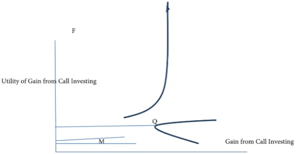
Given the strict band within which macroeconomic variables may vary, call op-tions on the Euro are likely to follow a distribution of small jumps. Figure 1
DOI: 10.4236/tel.2018.811148 2281 Theoretical Economics Letters Figure 1. Optimal trading levels for currency call options with put sales or small Jumps Equation (32) and Equation (33) expressions presented graphically.
preferences. At point M,in Figure 1, a highly risk-averse the trader is expected to always opt for a sure amount over a risky bet. The only sure call option strat-egy is to sell put options to a put buyer, at a premium = −Pt*n, where Pt= price of a single put option, and n = number of puts. There is no benefit to waiting for jumps to materialize, so the trader exits the market. In other words, the Coeffi-cient of Absolute Risk Aversion does not increase if there are additional risky opportunities for gain, as the rate of change in risk aversion remains at u'(c).
The Arrow-Pratt Coefficient of Risk Aversion [46],
( )
( ) ( )
1A c = −u c u c′′ ′ = (31) where, A(c) = an individual’s propensity to avoid risk, u(c) = the utility function of payoffs to an individual for accepting risk, with u'(c) and u''(c), as first and second derivatives. Small jumps in call option prices ensue with variations of the Euro within its narrow band. A risk-seeking trader has the utility function de-scribed in curve OF of Figure 1.
An increase in wealth (as promised by the gain from trading calls), results in the desire to increase wealth from further investment in call options with future jumps in euro values. An increase in the utility of wealth is a decrease in absolute risk aversion or A(c) < 0.In expanded form,
( )
{
( ) ( )
( )
2}
( )
2A c dc u c u c′ u c u c′
∂ = − − (32)
c =gain from an investment in call options, = [(Euro Value After the Jump − Exercise Price of the Call Option)] − Call Premium. This model posits that a trader will exercise the option and take the highest gain on a jump at the point at which the rate of change in the utility of wealth (defined in Equation (32)) equals the change in price of a call option along a Levy-Khintchine process (defined in Equation (33) below). This is the point of intersection of the utility function OF
DOI: 10.4236/tel.2018.811148 2282 Theoretical Economics Letters
( )
(
(
2 2(
)
)
)
€ei x t
θ
=exp t aiθ
−0.5σ θ
t +∫
ei xθ
t− −1 i x I xθ
t t< Π1 dx (33)As the aiθ quantity is a linear drift, and the 1 2 2 2
t
σ θ
term is a Brownian mo-tion, both of which are independent of jumps, they will be omitted from further consideration.The first jump in Figure 1 will be represented by
(
ei xθ t− −1 i x I xθ t t<1)
Πdx∫
The peak of this jump, at which the trader will realize the maximum gain from investing in the call option is the second derivative of the first jump.
The second derivative is
(
ei x i xI x tθ − θ < Π)
. Differentiating Equation (32) below,( )
( ) ( )
( )
2(
( )
)
2 x A c c u c u c′ u c u c′∂ ∂ ∂ ∂ = − − (34)
c =gain from an investment in call options, [(Euro Value After the Jump − Ex-ercise Price of the Call Option)] − Call Premium.At the minimum, the second derivative of the utility function = 0,
( )
2 0,or Euro value after the jump Exercise price of the call Call premium
u c′′ = −
= (35)
when the condition in Equation (35) is satisfied, a trader will make a trade, or exercise the call option, purchase the euro, and sell it for gain. The trader will continue to make similar trades until the gain < call premium, or the cost of purchasing the option is higher than the profit from the trade.
4.2. A Currency Call Option Distribution for Currencies with
Unconstrained Parameters and Small Jumps
Given that the macroeconomic variables may vary no more than 1 standard deviation from the mean, currency calls on currencies such as the Japanese yen, Australian dollar and Canadian dollar, may experience small jumps (See Section 3.2, for a description of the currency distribution). It is unlikely that very risk-averse traders who sell put options would trade options in these currencies, as even a 1 standard deviation change of macroeconomic variables would be considered to be excessively risky.
In Section 3.2, the optimal foreign currency value, xt,was presented as the so-lution to Equation (13).
Where, xt, the optimal foreign currency value, is the spot rate, or currency value at a point in time can also be the exercise price on a foreign currency call option as shown in the modification of Equation (35) below.
DOI: 10.4236/tel.2018.811148 2283 Theoretical Economics Letters
4.3. A Currency Call Option Distribution with Large Jumps
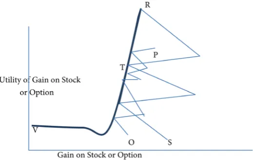
In Figure 2, a call option trader with a propensity for risk-seeking selects calls on highly volatile Mexican pesos or Turkish liras. Both the currency and calls have large jumps, but the calls having the lesser initial investment are riskier, and subject to larger jumps. In Figure 2, the jumps represented by OP are cur-rency (peso, lira, etc.) 2g2 (jumps, while those in SR are call option jumps. The trader’s risk preferences are presented in curve VR.The trader will purchase the option at the option premium. As call prices escalate beyond the currency price to a peak at, say, point T, the trader is satisfied that the option has achieved maximum gain, beyond any gain offered by the foreign currency.
Gain on the option Gain on the currency= (37) Or,
[
Final currency price Exercise price Call price]
Final currency price Currency purchase price− −
> − (38)
Currency function Gain on the option Levy Khintchine option function+ = − (39) If xt = value of foreign currency
(
)
2 1 2 2( )
2 2( )
( )
1 20.5sgn 8
? 1 1
t t t t it t
t
x b g xt h xt
CV X CP ei i I x
µ µ σ σ
θ δ θδ
− −
− ⋅ ∇ + ∇ + +
+ − − = − − >
∑
∑
∑
∑
∑
(40)
where, δ = jump size, CV = currency value, Ex = exercise price of the currency call option, CP = call premium.
At the point of earning the gain in the call option, T, in Figure 2, the Levy-Khintchine function is maximized, or, for a jump size, δ > 1, the maximum point is defined by the Right side of Equation (40).
5. Pricing Call Options
5.1. Pricing Currency Calls Meeting Euro Standards
[image:13.595.243.503.528.692.2]We will draw upon the currency distributions described in Section 3, as well as
DOI: 10.4236/tel.2018.811148 2284 Theoretical Economics Letters the call option distributions presented in Section 4, to develop expressions for pricing currency calls in this section. This includes combining the currency dis-tribution for euros in Section 3.1, with call option disdis-tributions on euros in Sec-tion 4.1 to develop the currency call pricing formula in SecSec-tion 5.1. Likewise, the currency distribution for stable currencies in Section 3.2 will be combined with call option distributions on stable currencies in Section 4.2, and in turn, curren-cy call pricing formulations in Section 5.3. The pattern continues for volatile currencies in Sections 3.3, 4.3, and 5.3. This paper employs the underlying asset pricing concept contained in [47] to formulate the price of call options t- on currencies meeting therestrictions of the European Union, based onthe distri-bution xt presented in Section 3.1. [47]’s Assumption A 6 states that:
The Value of A Contingent Claim such as a call option = (Gain From The Claim − Price Change Due To State Variables) + (Value of the Contingent Claim*. Distribution of the Contingent Claim),
Price of a call
Present value of currency Present value of exercise price Price change due to change in macroeconomy
Call premium Distribution of call
= − − + ∗
(
)
(
(
)
(
)
(
)
(
)
(
)
(
)
(
)
2 31 1 1
2 3
2 2 2
2 3
3 3 3
2 3 2 3
1 1 1 2 2 2
2 3
3 3 3 1 1 1
Forward rate 2 2
2 2 2 2
2 2 2 2
2 2 0.5
rdt rdt
t t t t t t
t t t t t t
t t t t t t
t t t t t t
t t t t t t t
C e e C x
x x
C x x
x L x
µ σ
µ σ
µ σ
µ σ µ σ
µ σ µ
− −
= ∗ − − ∗ − + ∆ − + ∆ Π + ∆
− + ∆ − + ∆ Π + ∆ − + ∆ − + ∆ Π + ∆
− ∗ − − Π − − Π
− − Π − + ∆ − + ∆ −
(
)
(
]
(
)
(
)
(
)
1 1 1 2 2 2
3 2 2 3 3
3 3 3
0.5 0.7
0.7 0.25
0.25 Call premium 1 1 d
t t t t t t
t t t t t t
t t
L x L x
L x L x
L x i x i xI x x
µ
µ
µ
µ
µ
θ
θ
− − − − + ∆ − + ∆ −
− − − − + ∆ − + ∆ −
− − − + ∗ − − <
Π
(41)
where, First term = Gain on exercise of the call option at the forward rate, or the present value of the gain (C*, currency value-forward rate) earned in the future at the foreign interest rate, rd, over the period, t.
Second and third terms = Objective function of Equation (8) that describes the pricechange in a currency call option due to change in macroeconomic va-riables from t to t, Δt. All L terms = Price change due to macroeconomic va-riables at t and t, Δt. L1, L2, L3 = Lagrange multipliers of constraints in Equation (8). Last term = Call premium*Levi-Khintchine call option distribution listed in Equation (33).
5.2. Pricing Currency Calls with Unconstrained Parameters and
Small Jumps
DOI: 10.4236/tel.2018.811148 2285 Theoretical Economics Letters (Value of the Contingent Claim*Distribution of the Contingent Claim),
(
)
(
)
(
)
Price of a call option
Present value of the currency
Present value of the exercise price of the option Price change due to change inmacroeconomy Call premium Distribution of the call option
= − −
+ ∗
while the present value of the currency − present value of exercise price is iden-tical to Section 5.1, other remaining terms need to be adjusted by the expressions in Section 3.2 and Section 4.2, for models with price stability and small jumps,
(
)
(
)
[
]
(
)
(
)
(
)
(
)
(
)
21 1 2 3 4 5 6 7
2 2
3 1 1 3 2 2
2 2
4 3 3 5 4 4
2
6 5 5 7
[ Forward rates (1 log[ 2 ]
[
[
rdt rdt
t t
t t t t t t t
t t t t t t
t t t t t t
t t t
C e e n x pxt x pxt
L x y x x x x x x x
L x y x L x y x
L x y x L x y x
L x y x L
µ
µ σ µ σ
µ σ µ σ
µ σ − − = ∗ − − −∂ + ∂ − ∂ ∂ + + + + + + − ∂ ∂ − − ∂ ∂ − − ∂ ∂ − − ∂ ∂ − − ∂ ∂ ⋅ −
− ∂ ∂x y x
(
6t−µt)
2 σ6t − L8∂x2 2p xt( )
(42)First term Gain on exercise of the call option at the forward rate, or the present value of the gain (currency value, C-forward rate) earned in the future at the foreign interest rate, rd, over the period, t.
Second term Objective function of Equation (13) that describes the price change in a currency call option due to change in macroeconomic variables, 1/L
terms Lagrange multipliers of constraints in Equation (15)-Equation (21), Last term Call premium*Levi-Khintchine call option distribution listed in Equation (33).
5.3. Pricing Currency Calls with Unconstrained Parameters and
Large Jumps
We adapt Ito’s Lemma [48] to specify the Price Change Due to Change in Ma-croeconomic Variables, omitting the diffusion term which = 0 for a Laplace dis-tribution,
(
2 3)
Price change due to change in macroeconomic variables=k T2 +2T (43) where k = constant, T = ending time period. 2 Equation (30) describes the value of currency in a Laplace distribution with large jumps, Substituting Equation(30) into Ito’s Lemma [48], Upon reduction, the value of currency in a Laplace dis-tribution based upon the change in macroeconomic variables from time = 1, to time = T, it follows that,
(
)
(
)
(
)
( )
( )
( )
2
2 4 5
1
2 2 2 2 2
Price of a call option Forward rate
2 1 1 8 8 Call premium 1 2sgn
8
rdt rdt
it it it it t t t
t t it t
CV e e
k b x b
g xt h xt CV Ex CP
σ σ σ σ µ µ
µ σ σ
− − − = ∗ − − + − + + ⋅ + ∗ − +
∑
∇ +∑
∇ +∑
+∑
+ − − (44)DOI: 10.4236/tel.2018.811148 2286 Theoretical Economics Letters
6. Conclusions
This paper has updated the sparse publications on stochastic processes in option pricing, most of which belong to the era of the 1980s and 1990s. Unlike papers that modify stock option pricing models, we recognize that stock and foreign currencies are fundamentally different. A share of stock represents ownership of a business, while foreign currency values are determined by macroeconomic forces and government policy. It follows that the values of stock and foreign currency vary in their movements over time. Stock distributions are typically lognormal with minimal skewness and kurtosis. Foreign currency distributions are discontinuous with jumps and skewness and significant fat-tails, or kurtosis. We create foreign currency distributions that account for skewness and kurtosis with high jump-based distributions such as the Laplace distribution. We im-prove on jump-diffusion and variance gamma distributions which account for small jumps, with Levy processes that explain large jumps.
From a practitioner standpoint, call options on each of the foreign currencies studied may be used to predict future currency values, so that importers who pay in foreign currencies, may protect their accounts payable from currency apprec-iation. In other words, if a currency rises in value, an importer who has to make a payment in that currency will experience higher expenses, unless they purchase a call option with low exercise price, that permits them to purchase the foreign currency at cheaper rates.
Future research should extend theoretical formulation beyond the three groups of currencies examined. Other currencies may include the Swiss franc, Australian dollar, Hong Kong dollar, Renminbi, baht, krona, and Singapore dol-lar. Our approach of first developing the formulation of the currency distribu-tion, followed by the option preserves the definition of an option as an instru-ment whose value is derived upon the foreign currency, so that is recommended over approaches that do not consider the distribution of the underlying foreign currency. Future research should also explore the use of risk preferences to iden-tify option distributions. Trader demand for call options is governed by risk-seeking. Risk-averse traders will seek modest gains, exiting when the risk of investment exceeds the coefficient of risk-aversion. Risk-takers with low coeffi-cients of risk-aversion will trade longer, until higher gains are achieved. Call op-tions assume a market of appreciating foreign currencies. How would traders react to a market of depreciating foreign currencies? Would they short sell the currency, exiting short selling due to regulatory restrictions, satisfying their de-mand for declining currency with put option purchases? How would those puts be priced? Future research must be directed to answering these questions.
Conflicts of Interest
DOI: 10.4236/tel.2018.811148 2287 Theoretical Economics Letters
References
[1] Feldman, R.S. (1985) Foreign Currency Options. Finance & Development, 22, 38-41.
[2] Bae, S.C., Sook, H. and Kwon, T.H. (2018) Currency Derivatives for Hedging: New Evidence on Determinants, Firm Risk, and Performance. Journal of Futures Mar-kets, 38, 446-467. https://doi.org/10.1002/fut.21894
[3] Bhagawan, P. and Lukose, J. (2017) The Determinants of Currency Derivatives Usage Among Indian Non-Financial Firms: An Empirical Study. Studies in Eco-nomics and Finance,34, 382-383.
[4] Wu, P.H. (1996) Derivative Strategies Used by United States Commercial Banks and Security Brokers for Foreign Exchange Risk Management. Unpublished Doctoral Dissertation, United States International University.
[5] Clark, E. and Mefteh, S. (2011) Asymmetric Foreign Currency Exposures and De-rivatives Use: Evidence from France. Journal of International Financial Manage-ment and Accounting,22, 27-45. https://doi.org/10.1111/j.1467-646X.2010.01044.x [6] Chong, L., Chang, X. and Tan, S. (2014) Determinants of Corporate Foreign
Ex-change Risk Hedging. Managerial Finance,40, 176-188. https://doi.org/10.1108/MF-02-2013-0041
[7] Mint (2011) Why Trade Foreign Currency Options. Mint,1.
[8] Szalay, E. (2014) Citadel Expands Into FX Market Making Promising to Match Tier I Bank Offerings, TX Week,4.
[9] Business Wire (2000) Gain Capital Expands Product Offering, Internet-Based For-eign Exchange Trading Service to Support Twenty Currency Pairs and Options Trading. Business Wire,1.
[10] Watt, M. (2014) Eurex Finalises FX Futures and Options Launch Date. FX Week,4. [11] Daal, E.A. and Madan, D.B. (2005) An Empirical Examination of the
Va-riance-Gamma Model for Foreign Currency Options. Journal of Business, 75, 2121-2152. https://doi.org/10.1086/497039
[12] Pitarbarg, V. (2005) A Multi-Currency Model with FX Volatility Skew. Working Paper.
[13] Schlogl, E. (2002) A Multicurrency Extension of the Lognormal Interest Rate Mar-ket Model. Finance and Stochastics,6, 173-196.
https://doi.org/10.1007/s007800100054
[14] Mikkelson, P. (2001) Cross-Country LIBOR Market Model. Unpublished Doctoral Dissertation, University of Aarhus.
[15] Ahn, C., Cho, D. and Park, K. (2007) The Pricing of Foreign Currency Options Under Jump Diffusion Processes. Journal of Futures Markets,27, 668-695. https://doi.org/10.1002/fut.20261
[16] Garman, M. and Kohlhargerr, S. (1983) Foreign Currency Options Values. Journal of International Money and Finance, 2, 231-237.
https://doi.org/10.1016/S0261-5606(83)80001-1
[17] Haque, M.A. and Saba, F. (2012) Currency Option Pricing Model Relevant to the Japanese Yen. Journal of International Business Research, 11, 119-128.
[18] Devereux, M.B. (1997) Real Exchange Rates and Macroeconomics: Evidence and Theory. The Canadian Journal of Economics,30, 773-808.
https://doi.org/10.2307/136269
DOI: 10.4236/tel.2018.811148 2288 Theoretical Economics Letters
Rate of the Indian Rupee. International Journal of Global Business Management,6, 49-57.
[20] Mirchandani, A. (2013) Analysis of Macroeconomic Determinants of Exchange Rate Volatility in India. International Journal of Economics and Financial Issues, 1, 172-179.
[21] Murari, K. and Sharma, R. (2013) OLS Modelling for Indian Rupee Fluctuations against the U.S. Dollar. Global Advanced Research Journal of Management Studies, 2, 559-566.
[22] Kama-Ainur, A. and Condrea, C. (2002) Some Empirical Evidence about the Effects of Macroeconomic Variables on the Exchange Rate in Romania. Transformations in Business & Economics,11, 435-450.
[23] Twarowski, K. and Kakol, M. (2014) Analysis of Factors Influencing Fluctuations in the Exchange Rate of the Polish Zloty Against Euro, Slovenia. Management Learn-ing and International Conference ProceedLearn-ings, 889-898.
[24] Kriljenko, C. and Habermeir, K. (2004) Structural Factors Affecting Exchange Rate Volatility: A Cross Section Study. International Monetary Fund, 5.
[25] Van Arle, B. and Hlouskova, J. (2000) Forecasting the Euro Exchange Rate Using Error Correction Models. Weltwirtschaftliches Archiv,136, 232-258.
https://doi.org/10.1007/BF02707687
[26] Ailinea, A.G., Milea, C. and Jordache, F. (2012) An Analysis Regarding the Fulfill-ment of the Nominal Convergence Criterion in the New Member States of the Eu-ropean Union in the Context of the Current Financial Crisis. Economy Transdiscip-linary Cognition,15, 14-21.
[27] Taylor, M.P. and Kim, H. (2008) Real Variables, Nonlinearity and European Real Exchange Rates. NBER International Seminar on Macroeconomics,5, 157-193. https://doi.org/10.1086/596004
[28] Branson, W.H., Haltunen, H. and Masson, P.R. (1977) Exchange Rate in the Short Run. European Economic Review, 10, 395-402.
https://doi.org/10.1016/S0014-2921(77)80002-0
[29] Solakoglu, M.N. (2000) Exchange Rate Volatility and International Trade. Unpub-lished Doctoral Dissertation, North Carolina State University, Raleigh.
[30] Chiang, T.C. (1985) The Impact of Unexpected Macro Disturbances on Exchange Rates in Monetary Models. The Quarterly Review of Economics and Business, 25, 49-60.
[31] McFarland, T.W., Pettit, R.R. and Sung, S.S. (1982) The Distribution of Foreign Exchange Rate Changes Trading Day Effects and Rate Measurement. Journal of Finance,37, 693-715.
[32] Calderon-Rossell, J.R. and Ben-Horim, M. (1982) The Behavior of Foreign Ex-change Rates. Journal of International Business Studies,13, 99-111.
https://doi.org/10.1057/palgrave.jibs.8490553
[33] Boothe, P. and Glassman, D. (1987) The Statistical Distribution of Foreign Ex-change Rates: Empirical Evidence and Economic Implications. Journal of Interna-tional Economics, 22, 297-319. https://doi.org/10.1016/S0022-1996(87)80025-9 [34] Engle, R.F. (1982) Autoregressive Conditional Heteroscedasticity With Estimates of
the Variance of United Kingdom Inflation. Econometrica, 50, 987-1007. https://doi.org/10.2307/1912773
DOI: 10.4236/tel.2018.811148 2289 Theoretical Economics Letters
[36] Chang, K.H. and Kim, M.J. (2001) Jumps and Time Varying Correlations in Daily Foreign Exchange Rates. Journal of International Money and Finance, 20, 611-637. https://doi.org/10.1016/S0261-5606(01)00007-9
[37] Akigray, V. and Booth, G.G. (1988) Mixed Diffusion Jump Process Modeling of Exchange Rate Movements. The Review of Economics and Statistics, 70, 631-637. https://doi.org/10.2307/1935826
[38] Merton, R.C. (1976) Option Pricing When Underlying Stock Returns Are Discon-tinuous. Journal of Financial Economics, 3, 125-144.
https://doi.org/10.1016/0304-405X(76)90022-2
[39] Bates, D.S. (1996) The Crash of ’87: Was It Expected ? Journal of Finance, 46, 1009-1044.
[40] Campa, J.M., Chang, P. and Reider, R.L. (1998) Implied Exchange Distributions: Evidence from OTC Options Markets. Journal of International Money and Finance, 17, 117-160. https://doi.org/10.1016/S0261-5606(97)00054-5
[41] Carr, P.H., Geman, H., Madan, D. and Yor, M. (2002) The Fine Structure of Asset Returns: An Empirical Investigation. Journal of Business, 75, 305-332.
https://doi.org/10.1086/338705
[42] Madan, D., Carr, P. and Chang, E. (1998) The Variance Gamma Process and Op-tion Pricing. European Financial Review,2, 79-105.
https://doi.org/10.1023/A:1009703431535
[43] Hormander, L. (1990) The Analysis of Partial Differential Operators. Springer, New York.
[44] Dhrondt, J.K.G. (1996) An Introduction to Dynamics of Colloids. Elsevier, Ams-terdam.
[45] Ottinger, H.C. (1996) Stochastic Processes in Polymeric Fluids. Springer-Verlag, Berling-Heidelberg.
[46] Pratt, J.W. (1964) Risk Aversion in the Small and the Large. Econometrica, 32, 122-136. https://doi.org/10.2307/1913738
[47] Cox, J.C., Ingersoll, J.E. and Ross, S.A. (1985) An Intertemporal General Equili-brium Model of Asset Prices. Econometrica, 53, 363-384.
https://doi.org/10.2307/1911241