Simulationofwater flow glazing for hvac using polymorphic components andbond graphs

SIMULATIONOFWATER

COMPONENTS ANDBOND GRAPHS

1,*

_{Fernando del Ama Gonzalo}

1

_{Alfaisal University P.O. Box 50927, Riyadh, Kingdom of Saudi Arabia}

2

_{School of Aeronautical and Space Engineering, Technical University of Madrid, Pza.}

Cardenal Cisneros, 28040, Madrid, Spain

ARTICLE INFO ABSTRACT

Energy consumption in

consumption. In the US, 30% of all energy consumed by commercial buildings is related to inefficient operation of building equipment.

construction of buildings that do not consume energy. US Department of Energy has been developing for many years the Energy

very complex cl

water-flow windows. In other occasions, the mathematical models do not correspond to reality. For all these reasons,

system simulations. Much effort is involved in codifying all of these configurations, even in the case of Energy

abstractions, defined as components lin system’s components

minimum effort. A list of components or nodes define a list of arcs that link the different components in an automatic way.

Copyright © 2015 Fernando del Ama Gonzalo and Juan Antonio Hernández

License, which permits unrestricted use, distribution, and reproduction in any medium, provided the original work is properly cited.

INTRODUCTION

The building’s climate control is comprised of a set of complex systems, in which many factors take action. Due to the rise of energy price over the last few years, the codes governing construction and buildings’ conditioning are imposing devices that allow for energy production by renewable sources. The guideline 2010/31/UE of the European Parliament regarding energy efficiency in buildings specifies that 20% of energy produced in Europe must come from renewable sources. This entails that buildings, as final energy consumers, must tend to integrate devices that produce energy for climate control and lighting. The cost of climate control equipment is high.It is necessary to develop prior simulation systems able to guarantee that the decisions made in the project phase are optimum in terms of providing comfort to the occupants wit the minimum energy expense (Yu. and van Paassen, 2004).

*Corresponding author: Fernando del Ama Gonzalo,

Alfaisal University P.O. Box 50927, Riyadh, Kingdom of Saudi Arabia.

ISSN: 0975-833X

Article History:

Received 10th _{April, 2015} Received in revised form 26th _{May, 2015} Accepted 07th _{June, 2015} Published online 31st _July,2015

Key words:

Water Flow Glazing,

Energy Simulation in Buildings, Bond Graphs

Citation:Fernando del Ama Gonzalo and Juan Antonio Hernández components andbond graphs”, International Journal of Current Research

RESEARCH ARTICLE

SIMULATIONOFWATER-FLOW GLAZING FOR HVAC USING POLYMORPHIC

COMPONENTS ANDBOND GRAPHS

Fernando del Ama Gonzalo and

_{Juan Antonio Hernández}

Alfaisal University P.O. Box 50927, Riyadh, Kingdom of Saudi Arabia

of Aeronautical and Space Engineering, Technical University of Madrid, Pza.

Cardenal Cisneros, 28040, Madrid, Spain

ABSTRACT

Energy consumption in buildings represents 40% of the European Union’s whole energy consumption. In the US, 30% of all energy consumed by commercial buildings is related to inefficient operation of building equipment. Horizon 2020 Program encourages the design and construction of buildings that do not consume energy. US Department of Energy has been developing for many years the Energy Plus: a simulation code that allows energy consumption simulations of complex climate control systems. However, this program does not address elements such as flow windows. In other occasions, the mathematical models do not correspond to reality. For all these reasons, it is necessary to develop parallel software for the evaluat

system simulations. Much effort is involved in codifying all of these configurations, even in the case of Energy Plus. The present work consists of the development of a simulation code based on abstractions, defined as components linked among each other by graphs. Once modeling each of the system’s components is done, the energy simulation of a specific installation

minimum effort. A list of components or nodes define a list of arcs that link the different components in an automatic way.

Fernando del Ama Gonzalo and Juan Antonio Hernández. This is an open access article distributed under the Creative Commons Att use, distribution, and reproduction in any medium, provided the original work is properly cited.

The building’s climate control is comprised of a set of complex in which many factors take action. Due to the rise of energy price over the last few years, the codes governing construction and buildings’ conditioning are imposing devices that allow for energy production by renewable sources. The the European Parliament regarding that 20% of energy produced in Europe must come from renewable sources. This entails that buildings, as final energy consumers, must tend to or climate control and The cost of climate control equipment is high.It is necessary to develop prior simulation systems able to guarantee that the decisions made in the project phase are optimum in terms of providing comfort to the occupants with the minimum energy expense (Yu. and van Paassen, 2004).

Fernando del Ama Gonzalo,

Alfaisal University P.O. Box 50927, Riyadh, Kingdom of Saudi

Simulation models have therefore to be designed in such a way to make easier the understanding of the user

Lebrun, 2008). The mathematical simulation of these systems requires several levels of abstraction. First, the real simulation is simplified by means of a schematic diagram of the energy installations. Later, each element of the installation is defined as a set of components. A complex set of interrelated problems can be brokendown into smaller discrete units

Kropman, 1997). A series of inputs and outputs define each component. In the case of a

components can have inputs and outputs of fluids (water, air, cooling fluids with low boiling points…) as well as inputs and outputs of heat flows due to the convective energy exchange with other components at different temperat

tools for HVAC design and analysis can be categorized with respect to the problems they are meant to deal with. Although some tools can handle several problems, they do tend to be investigated in isolation from each other (Trcka and Hensen, 2010). Reference and detailed models of HVAC components may help a lot in the commissioning process, among others for functional performance testing (Visier and Jandon, 2004). These detailed models may also help a lot in the daily system management for fault detection and diagnosis (Jagpal, 2006).

International Journal of Current Research

Vol. 7, Issue, 07, pp.18349-18355, July, 2015

Fernando del Ama Gonzalo and Juan Antonio Hernández 2015. “Simulationofwater-flow glazing for hvac using polymorphic International Journal of Current Research, 7, (7), 18349-18355.

FLOW GLAZING FOR HVAC USING POLYMORPHIC

Antonio Hernández

Alfaisal University P.O. Box 50927, Riyadh, Kingdom of Saudi Arabia

of Aeronautical and Space Engineering, Technical University of Madrid, Pza.

the European Union’s whole energy consumption. In the US, 30% of all energy consumed by commercial buildings is related to Horizon 2020 Program encourages the design and construction of buildings that do not consume energy. US Department of Energy has been developing Plus: a simulation code that allows energy consumption simulations of imate control systems. However, this program does not address elements such as flow windows. In other occasions, the mathematical models do not correspond to reality. For it is necessary to develop parallel software for the evaluation by means of energy system simulations. Much effort is involved in codifying all of these configurations, even in the case Plus. The present work consists of the development of a simulation code based on ked among each other by graphs. Once modeling each of the specific installation scheme requires a minimum effort. A list of components or nodes define a list of arcs that link the different components

is an open access article distributed under the Creative Commons Attribution use, distribution, and reproduction in any medium, provided the original work is properly cited.

Simulation models have therefore to be designed in such a way r the understanding of the user (Bertagnolio and The mathematical simulation of these systems requires several levels of abstraction. First, the real simulation is simplified by means of a schematic diagram of the energy Later, each element of the installation is defined as a set of components. A complex set of interrelated problems can be brokendown into smaller discrete units (Wim and . A series of inputs and outputs define each component. In the case of a climate control system, the components can have inputs and outputs of fluids (water, air, cooling fluids with low boiling points…) as well as inputs and outputs of heat flows due to the convective energy exchange with other components at different temperatures. Existing tools for HVAC design and analysis can be categorized with respect to the problems they are meant to deal with. Although some tools can handle several problems, they do tend to be investigated in isolation from each other (Trcka and Hensen, 2010). Reference and detailed models of HVAC components may help a lot in the commissioning process, among others for functional performance testing (Visier and Jandon, 2004). These detailed models may also help a lot in the daily system ult detection and diagnosis (Jagpal, 2006).

OF CURRENT RESEARCH

The multilayer programming allows the simulation of complicated physical systems. The basicidea of this paradigm is based on the construction of abstractions, with a hierarchy related to their functionality (Hernández and Zamecnik, 2001). Graphs represent structures of differentbuilding energy systems and behaviors of buildingenergy moving in these structures. (Tsai and Gero, 2006). The physical components that make up the system are: Water-flow glazing. It consists of two glass layers, between which a water-flow chamber exists. Itcan be used either in the exterior to capture solar radiation and heat water, or in the interior, to emit heat if the water is flowing at a higher temperature than that of the interior air.

A heat pump uses a cooling fluid with a low boiling point. This thermal machine allows the transfer of energy by heat, as deemed necessary. To achieve this, an electric input is required. A buffer tank is a large volume of water with several inputs and outputs. It can serve as an energy-storing device, or to dissipate that energy when there is an excess of heat in the circuits of the water-flow glazing. The plate heat exchangers are devices that allow the transfer of calorific energy between all the previous devices. They are composed of thin metal plates, with a great surface for heat exchange between fluids that flow through each of these plates.

MATERIALS AND METHODS

Climate control systems in buildings

To achieve a feeling of comfort in the interior of a building, the temperature and relative humidity must be controlled. For this, it is necessary to provide enough energy to compensate the gains and losses produced through the enclosing elements and to allow the ventilation of the interior air. In the building studied for this paper, both solar energy and a water-to-water heat pump provide the energy needed for all the system. Solar energy is captured by means of water-flow glazing located in the exterior skin. Water-flowglazing located in inner partitions transfers heat to the interior of the building by means of radiation and convection.

Energy sources for this project are the sun and a water to water heat pump. Water-flow glazing placed on the roof heats up the water and a heat plate exchanger transfers energy either to a buffer tank or to a domestic hot water tank. The heat pump works when solar energy is not enough to reach the required temperature. Figure 3 shows the different components of the building and heat transfers.

Thermal simulation of the climate control system

The goal of this section is to put together all the algebraic or differential equations of the elements that make up the building’s climate control system, in order to obtain the global performance of the system. The idea that lies under this is to create a programming abstraction of the particular element in the climate control system. This way, all the elements or components of the system have a set of equations, packed in a state vector, which contains all the degrees of freedom of the system as a whole. Therefore, we have a set of ordinary differential equations, with their initial conditions constituting a Cauchy Problem.

call Solution_Cauchy_Problem (Domain= Time_Domain, Initial_condition = IC_Building,

System_of_equations = Building_equations, Outputs = Building_graphs)

The key lies now in creating a software functionality that will assemble the equations of each element and make the hydraulic connections between the different elements, automatically.

Definition of the components

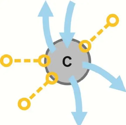
From the programming point of view, the components of the systems are black boxes, or open systems characterized by an input and an output, as well as by a surface that exchanges heat with other components or with an exterior environment. However, from the point of view of the ruling equations, it is important to be aware of their internal nature. This double need motivated us to consider the components as polymorphic objects, in order to make the software treatment much simpler.

Figure 1. Definition of a Bond Graph system component. Blue arrows represent inlet and outlet fluids. Dashed lines represent energy interchanges with other components by means of radiation and convection.

This is to say, a water tank can be treated generally as an open generic system when linking its output with the input of another component, or as a water tank with the singularity of its performance. A component is defined as the following object:

type component

integer :: variables

type (connector) :: inlet(:), outlet(:)

type (interface) :: interfaces(:)

character (len=*) :: name

endtype

A component is characterized by its degrees of freedom or number of independent variables, a set of input connectors, a set of output connectors and a set of interfaces that allow the exchange of heat with the exterior, or among components.

type connector

real, pointer:: T

real, pointer:: m

end type

typ einterface

real, pointer:: Q

endtype

The building’s climate control system is comprised of a set of polymorphic components, a set of circuits and a list for the connections of the different borders. The different polymorphic components can be water tanks, Water Flow windows, heat exchangers, etc.

type Building

type (Polymorphic_Component), allocatable :: Components(:)

type (arc_list), allocatable :: Circuits(:), Interfaces

real, allocatable :: Q(:)

endtype

type :: Polymorphic_Component

class(*), pointer :: p

endtype

typearc

character(len=*) :: source, target

endtype

typearc_list

type (arc), allocatable :: name(:)

endtype

The different circuits linking these components can be the primary, secondary, tertiary (and so on) hydraulic circuit. In turn, each circuit is characterized by a set of arcs, which are pairs of names that link components. Lastly, the list for the connection of the components’ borders allows heat transfer from one circuit to another.

This way, any climate control system of a building can be defined through the components it is made of. Links between the components’ inputs and outputs are determined by the circuits, and heat transfers between components are determined by the list of border connections.

Water tank for the accumulation of energy

A water tank is defined by a border, which can exchange heat with the exterior, as well as by an input and an output which exchange water mass. The non-uniform water temperature inside the tank and the thermal mixing processes are ruled by the Navier-Stokes equations. However, if the temperature of the water is considered to be uniform, the interior temperature of the tank is ruled by an ordinary differential first order equation. What is important to mention is that, regardless of the mathematical model adopted for the deposit, the abstraction of the proposed simulator in this work does not change. For the simulator, a tank is an additional component, with a set of N ordinary differential equations. With this model, the tank can be defined as the extension of a component. It is an object that inherits the properties and the form of a component.

type, extends(Component) :: Water_tank

real, pointer :: T

real :: Tdot

real :: c = 4180

real :: flow = 30 ! l/min

real :: Volume = 15 ! m3

real :: Surface = 20 ! m2

real :: density = 1000 ! kg/m3

real :: hext = 10 ! W/m2K

contains

procedure :: Constructor =>Constructor_Water_tank

procedure :: Equations =>Equations_Water_tank

procedure :: Ini =>Ini_Water_tank

endtype

The Buffer-Tank object is characterized by its temperature T (the only independent variable), by all the properties of a component, and by the specific properties that define it: mass, specific heat… Furthermore, the water tank includes its constituent equations, as well as its initial conditions.

Water-flow glazing

The complexity of the mathematical model for a water-flow window depends on the level of physical approach one wants to obtain. In the simplest case, the window can be treated as an open system that exchanges heat with the exterior through its defining surfaces and through the convective flow associated to its input and output. This way, the uniform temperature of the window is considered to be ruled, as in the case of the tank, by an ordinary differential first order equation.

In contrast to this simplified case, the heat transfer produced in each window part (glass panes, water chamber and air chambers) could be simulated in a generic manner. This way, the heat transfer mechanisms are: radiation, conduction and convection. The heat equation for the glass panes and the Navier-Stokes equations for the water and air chambers govern the temperature evolution of the windows. These equations, which constitute a set of partial differential equations, must be completed with boundary and initial conditions that come from the different layers. The problem posed is of extreme difficulty.

In the middle ground between these two models, a simpler model could be posed for the water and air chambers, as well as for the glass panes. Due to the fact that the air chamber has little thermal inertia, it is modeled by an algebraic equation with a transfer coefficient that links the heat transported by the chamber from one glass pane to the other. Furthermore, if the water temperature is considered uniform, the water temperature in the chamber would be ruled by an ordinary differential equation.

Figure 3. Definition of the energy management system by means of graphs. Roof water-flow glazing (H); Heat plate exchangers (H1A-H1B H2A-H2B, H3A-H3B y H4A-H4B); Interior (I); Exterior (E); Electric input (W); Buffer Tank (BT); Domestic hot water tank (DHW); Heat plate exchanger (ACS); Heat pump defined by two heat plate exchangers (H5A-H5B y H6A-H6B) and a compressor (C).

Blue arrows represent fluid circuits. Red dashed lines represent heat exchange by means of convection and radiation

In the case of the glass panes, the heat transfer is considered perpendicular to the pane, and its temperature is ruled by the one-dimensional, non-steady heat equation. Even in this mid-level model, there is great difficulty in simulating an isolated window. If we think of the complexity of a building’s complete climate control system, one can understand the need to make an effort of abstraction to tackle the challenge. In this case, the definition of the type of water-flow window is more complex. A window is an extension of a component, formed by polymorphic layers of water, air or glass.

type, extends(Component) :: Waterflow_Window

type (Polymorphic_Pointer), pointer :: Layer(:)

real, allocatable :: T_I(:)! temperatures at interfaces between

layers

real, allocatable :: alpha_I(:)! absorption at interfaces (PVB)

type (Surface) :: S

contains

procedure :: Constructor => Constructor_Waterflow_window

procedure :: Equations => Equations_Waterflow_window

procedure :: Ini =>Ini_Waterflow_window

endtype

Moreover, the water-flow window includes the equations that govern the window’s temperature. These equations are obtained by grouping the equations for each of the layers. The water-flow windows taking part in the system are, in principle, different among each other. The object defined before does not apply for all of them. Even for the simple model chosen previously for the window, the problem is not easy. The window is a set of polymorphic layers: glass, water and air. Determining the temperature in each of them demands the integration of at least one differential equation, with boundary conditions that depend on the rest of the layers. To conduct this process, the conservation equations of all the layers’ boundariesare posed in a generic manner, and the resulting system is solved by a Newton. Once the values of the temperatures in the intermediate phases are determined, the heat flows in the interior points of each layer can be calculated.

functionEquations_Waterflow_window( W )

class (Waterflow_window), target :: W

! ** Solve temperatures at interfaces i = 0....N, unkonwns:

call Newton( F_Interface, W % T_I )

! ** Energy balance for each layer

doi = 1, Nlayers

select type ( A => W % Layer(i) % p )

type is (Water_layer)

Equations_waterflow_window(:) = A % Equations( T_agua, ie)

type is (Glass_layer)

Equations_waterflow_window(:) = A % Equations(ie)

type is (Air_layer)

Equations_waterflow_window(:) = A % Equations()

end select end do contains

functionF_Interface(T_interface)

Q(0, 1) = q_ext Q(N, 2) = q_int

doi=1, N

select type ( A => W % Layer(i) % p )

type is (Glass_layer)

Qb = A % Fluxes()

type is (Water_layer)

Qb = A % Fluxes(Inclination)

type is (Air_layer)

Qb = A % Fluxes(Inclination)

end select

Q(i-1,2) = Qb(1) Q(i,1) = Qb(2)

end do

F_Interface(:) = Q(:,1) - Q(:,2) + W % alpha_I(:) * ie

end function end function

Plate heat exchanger

Generally, the thermal inertia of a plate heat exchanger is small when compared to the thermal inertia of the system. Therefore, the set of equations ruling the heat exchange process can be considered stationary or quasi-stationary.

On the other hand, the design of the exchanger is strongly linked to its function and, consequently, to its mathematical model. The company that has developed the heat exchanger, due to their knowledge of the product, offers a simplified model made up of two algebraic non-linear equations that relate the inputs and outputs of the primary and secondary circuits.

Circuits

CIRCUIT 1 CIRCUIT 2 CIRCUIT 3 CIRCUIT 4

SOURCE I E H H1A H H2A H1B H3A BT

TARGET E I H1A H H2A H H3A BT H1B

CIRCUIT 5 CIRCUIT 6 CIRCUIT 7 CIRCUIT 8

SOURCE H4B R H6B BT H H2A H5B C H6A

TARGET R H4B BT H6B H2A H C H6A H5B

CIRCUIT 9

SOURCE H4A H3B ACS H5A TARGET H3B ACS H5A H4A

Interfaces

The installation’s schematic diagram through the connection of components

The idea now consists of linking together components in a schematic diagram of the thermal climate control system. From a mathematical point of view, these connections constitute a graph. The nodes or vertices of the graph are the components and the arcs or lines of the graph can either be the hydraulic pipes that link the elements or components of the system, or the virtual bonds between components which symbolize the heat transfer among them. This way, a set of components or nodes define the graph, and by a set of pipes or arcs that link components together.

All pipes linking pairs of components are considered. Once all the inputs and outputs are connected, all the components’ borders or surfaces have to be linked too in order to indicate the heat flow between them. Therefore, a graph can represent the flow of water from a closed circuit, and the flow of heat between components is represented by another graph, superimposed to the first. The connections of inputs and outputs of the components, as well as the connections between borders, can be done in a generic manner without knowing if we are dealing with a window or a tank. In the following pseudocodes, it is shown through pointers how these connections are carried out. The input temperature of a component is pointed as the output temperature of another component. Being the same variable, when the output temperature changes the input temperature changes as well.

subroutine Connections(inlet, outlet, C)

select type ( A => C(outlet) % p )

class is (Component)

select type ( B => C(inlet) % p )

class is (Component)

! inlet of the component A points to outlet of B A % inlet % T => B % outlet % T

A % inlet % m => B % outlet % m

end select end select end subroutine

Likewise, the connection is done between components that are in contact by their surfaces and exchange heat through them.Both the connections between inputs and outputs and the connections between the surfaces of the different components are carried out once, in the initialization of the problem. These connections guarantee the continuity of superficial and input/output temperatures for the components that take part in the system or building. The simulation of the whole problem consists of integrating the Cauchy problem or initial conditions that result from gathering all the constituent equations of the system. Once again, this process can be carried out in an automatic manner by means of the following pseudocode.

subroutineBuilding_equations(t, U, F )

B % Heat_fluxes_at_interfaces(t)

doi=1, Nc

select type( A => B % Component(i) % p )

class is (Component)

select type( A => B % Component(i) % p )

type is (Water_tank)

F(:) = A % Equations(t)

type is (Waterflow_window)

F(:) = A % Equations(t)

type is (Air_Zone)

F(:) = A % Equations(t)

end select end select enddo

end subroutine

Firstly, the heat flows between the different interfaces of the system’s components are obtained; this makes up a system of M equations, where M stands for the number of interfaces. Each of these equations dictates that the flow from the right matches the flow from the left of the interface. Each of the components is coupled with the rest through border conditions, which are the heat flows in the interfaces. In this subroutine, U (t) represents the system’s state vector and F (U,t) represents its variation throughout time. This gives a Cauchy problem with N dimensions. The independent variables of the system, or degrees of freedom, are the independent variables of each and every component. In the initialization, the independent variables of each component are pointed to a part of the state vector. Finally, the result of the equations of each of the components is packed in a column vector F(:) and the problem is sent to a temporal integrator.

DISCUSSION

Climate control systems in buildings are becoming increasingly more complex. Their mathematical approach requires conceiving them as thermodynamic systems formed by open subsystems. In this paper, a component has been defined as an open system characterized by its inputs, outputs and a non-permeable surface through which heat can be transferred among other components. This way, the different subsystems of a climate control system can be considered as components or open systems. The different components exchange energy with other components by means of two very different mechanisms: (i) forced energy transport by means of a fluid associated to its input and output and (ii) the thermal exchange through the borders of each component. Blue directional arcs linking different components indicate the energy transport in a flowing fluid. Red non-directional arcs indicate the thermal exchange. This way, a graph is comprised of different components that take part in the system, together with different blue and red arcs.

The introduction of graphs in this type of climate control systems has the following benefits:

 It enables a much faster explanation of climate control

systems. The paths that the heat can follow in the energy transfer become evident. Accordingly, graphs show the energy strategy of the system without a need to address the more complicated physical mechanisms of heat transfer.

 It allows the detection, in a design phase, of errors in the

topology of the system. Open loops or unused paths of energy transfer.

 It makes the simulation of very complex installations possible, without the need to write a specific program for it.

This article has described a simulator based on polymorphic components, which allowsto determine the heat transfer between the components of a generic graph. To simulate a particular installation, the user simply introduces the list of components and the list of arcs that define the given installation.

Acknowledgement

The work described in this article was supported by the 2015 Alfaisal University Internal Reseach Grants (Water flow glazing and absorption chillers for solar cogeneration in buildings).

REFERENCES

Bertagnolio, S. and Lebrun, J. 2008. Simulation of a building and its HVAC system withan equation solver: Application to benchmarking. Building Simulation: AnInternational Journal, 1(3): 234-250.

Hernández, J.A. andZamecnik, M.A. 2001. FORTRAN 95: Programación Multicapa para la Simulación de Sistemas Físicos, Publisher ADI, Madrid.

Jagpal R. 2006. International Energy Agency – Energy Conservation in Buildings andCommunity Systems Annex 34: Computer Aided Evaluation of HVAC System Performance. Synthesis Report.

Trcka, M. and Hensen, J. L. M. 2010. Overview of HVAC system simulation. Automation in Construction, vol. 19, no. 2, pp. 93-99.

Tsai, J.J. and Gero, J.S. 2006. Qualitative archi bond graphs for building simulation of people behavior and energy variation. Proceedings of the Second National IBPSA-USA Conference Cambridge, MA: 277–284.

Visier, J.C. and Jandon, M. 2004. International Energy Agency – Energy Conservation in Buildings and Community Systems Annex 40: Commissioning of Building HVAC Systems for Improved Energy Performances. Synthesis Report.

Wim, Z. and Kropman, B.V. 1997. Design and simulation of HVAC systems with bond graph's. Proceedings of the

bi-annual international IBPSA Building Simulation

Conference and Exhibition held at Prague, Czech Republic.

Yu, B. and van Paassen, A.H.C. 2004. Simulink and bond graph modelingof an air-conditioned room. Simulation Modelling Practice and Theory, 12: 61–76.