Control of Uncertain Fuzzy Networked Control
Systems with State Quantization
Magdi S. Mahmoud
Systems Engineering Department, King Fahd University of Petroleum and Minerals, Dhahran, Saudi Arabia Email: [email protected]
Received September 11, 2011; revised October 11, 2011; accepted October 18,2011
ABSTRACT
T
he problem of robust control for uncertain discrete-time Takagi and Sugeno (T-S) fuzzy networked control sys-tems (NCSs) is investigated in this paper subject to state quantization. By taking into consideration network induced delays and packet dropouts, an improved model of network-based control is developed. A less conservative de-lay-dependent stability condition for the closed NCSs is derived by employing a fuzzy Lyapunov-Krasovskii functional. Robust fuzzy controller is constructed that guarantee asymptotic stabilization of the NCSs and expressed in LMI-based conditions. A numerical example illustrates the effectiveness of the developed technique
.
Keywords: Networked Control; Fuzzy Systems; Discrete Time-Varying Delay; Linear Matrix Inequality (LMI)
1. Introduction
Fuzzy system models have been widely adopted to rep-resent certain classes of nonlinear dynamic systems fol-lowing the T-S fuzzy model [1]. Since then there have been several approaches for the study of stability analysis and robust controller synthesis using the so-called paral-lel distributed compensation (PDC) method for uncertain nonlinear systems [2,3]. Sufficient conditions have been derived based on the feasibility testing of a linear matrix inequality (LMI) in [4-7] and extended for classes of nonlinear discrete-time systems with time delays in [8-10] via different approaches. Recently, much attention has been paid to the stability issue of network based control systems [11]. Several results pertaining to the analysis and design of networked control systems (NCSs) en- hanced their wide benefits such as reducing system wir- ing, ease of system diagnosis and maintenance, and in- creasing system agility, to name a few. However, com- munication network in the control loops gave rise to some new issues, especially the intermittent losses or delays of the communicated information due to use of a network, which imposes a challenge to system analysis and design. To address this challenge, many results have been developed in consideration of network-induced de- lay and packet dropout [12-18], with focus on stability analysis and controller design with random delays.
Further consideration of the communication of the NCSs over the channel emphasized the importance of signal quantization, which has significant impact on the
performance of NCSs. In this regard, the problem of guaranteed cost control and quantized controller design were discussed in [17] by using two quantizers in the network both from sensor to controller and from control-ler to actuator, and the network-induced delay and data dropped were considered as well.
Recent advances converted the quantized feedback de-sign problem into a robust control problem with sector bound uncertainties, [11] and [16-18]. Parallel investiga- tions to the class of switched discrete-time systems with interval time-delays were developed in [19-23].
Despite the potential of these developments, the prob-lem of how to analyze the stability of nonlinear NCSs with data drops still open. On the other hand, most in-dustrial plants have severe nonlinearities, which lead to additional difficulties for the analysis and design of con-trol systems. Though some issues on nonlinear NCSs have been investigated [23,24], limited work has been found on robust state feedback controller design of
networks for fuzzy systems with consideration of both network conditions and signal quantization.
The guaranteed cost networked control and robust
x
network induced-delay and packet dropout. However, they do not quantize the signals. The foregoing facts mo-tivate the present study.
In this research work, we address the robust
t 1
state feedback control problem for discrete-time networked systems with state quantization and disturbances. The T-S fuzzy systems with norm-bounded uncertainties are utilized to characterize the nonlinear NCSs. Since the computation available is often limited, the quantized feed- back controller is designed under consideration of effect of network-induced delay and data dropout, the em- ployed quantizer is time-varying. By using a new fuzzy Lyapunov-Krasovskii functional (LKF), we provide a sufficient LMI-based condition for the existence of a fuzzy controller. A numerical example shows the feasi-bility of the developed technique.
Notations and facts: In the sequel, the Euclidean norm is used for vectors. We use W and W to de-note the transpose and the inverse of any square matrix
, respectively. We use to denote a symmetric positive definite (positive semi-definite, nega-tive, negative semi-definite matrix W and
W W > 0 ( , <, 0)
I to de-note the identity matrix. Matrices, if their dimen-sions are not explicitly stated, are assumed to be com-patible for algebraic operations. In symmetric block ma-trices or complex matrix expressions, we use the symbol () to represent a term that is induced by symmetry.
n n
Fact 1: For any real matrices
1, 2 and
3 with appropriate dimensions and
3t 3I, it follows that1 1
1 3 2 2 3 1 1 1
t t t t
2 2, 0t
0
T
,
S k
th
j
is jn, then
k M
Sometimes, the arguments of a function will be omit- ted when no confusion can arise.
2. Problem Description
A typical networked control system typically has a clock- driven sampler and a quantizer, controller, a zero-order hold (ZOH) which is event-driven. The sampling period is assumed to be with the sampling instants as
k . The plant belongs to class of uncertain
discrete-time systems where the parametric uncertainties are norm-bounded.
, = 1,
In what follows, we consider that this class is repre-sented by Takagi-Sugeno fuzzy model composed of a set of fuzzy implications, and each implication is expressed by a linear system model. The rule of this Takagi- Sugeno model has the following form:
1 1
Rule j: If( ) isk Mj ,andn
1 =
j
j
j
,x k A x k Bu k w k
,j
= j
j
y k C x k D u k w k
= , M, 0 , = 1, 2, ,
k k k j r (1)
where 1 k ,2 k
,,n
k are the premise vari-ables, each Mjm
m= 1, 2,n
r
nx k
are the fuzzy sets, is the number of if-then rules and is the state vector, u k
m is the control input, y k
qis the output, w k
p is the disturbance input which belongs to 2
0,
and M indicates the maximumallowable signal transmission delay. The uncertain ma-trices Aj,,j are represented by:
=
j j j j j j
j j j j j j
j j j
j j j
A B A B
C D C D
A B
C D
1
1 2 3
2
= ( )
j j j
j j j
j
j j j j
j
A B
C D
M
F k N N N
M
(2)
, , , where the matrices A Bj j j
, , , ,
describe the nominal dynamics and M1j M2j N1j N2j N3j are known
con-stant real matrices with appropriate dimensions. The ma-trices F kj
are unknown time-varying and satisfying
, , 0t
Fj k F kj I k
=1 =1
1 =
=
r
j j j j
j
r
j j j j
j
.
Using a center average defuzzifier [1], product infer-ence, and incorporating fuzzy “blending”, the fuzzy sys-tem under consideration can be cast into the form
x k f k A x k B u k w k
y k f k C x k D u k w k
(3)
where
=1
=1
= ,
= j
j r
j j
n
j jm m
m
F k
f k
F k
k M k
(4)
F
m
jmM k is the grade of membership of where
m k in Mjm. In the sequel, we assume that
=1
0, = 1, 2, , , > 0, 0 r
j j
j
F k j r
F k k
=1
0, = 1, 0
r
j j
j
f k
f k k and thereforeOur objective in this paper is to design a fuzzy
state feedback controller with state quantization.
3. Controlled Fuzzy System
In what follows, we proceed to consider establish the main result for the uncertain discrete-time fuzzy net-worked control systems described by (3) and design the quantized fuzzy state feedback controller. We
con-sider a limited capacity communication channel and for reducing the amount of data rate of transmitting in the network, which led to the increase quality of service of the network, we assume that the state vector
x k
is measurable. The state signal from sensor to the controller is quantized via a quantizer, and then transmitted with a single packet. To reflect realty, network-induced time delay is modeled as an input delay and the packet drop-out will be considered.
3.1. State-Feedback Control
In effect, we seek to design the state-feedback controller:
=K x d T
k
= ,
u k g k k
(5)
where g k is the feedback law to be defined in the sequel and dk,
k= 1, 2, 3,
are some integers such
that d d d1, 2, 3,
1, 2, 3,
= =
d T k kd T k k
> 1
d d
< ,
d d
1 ,
, 1
k d d T k
T k
. Introduce
k =k d Tk which contains the information of packet dropouts and improper packet sequence in the control signal. Note that k k .
It has been pointed out in [19] that when
1
k k there would be no packets dropout and the
case k1 k represents continuous packets lost. In
addition, when k1 k the new packet reaches the
destination before the old one. This case might lead to a less conservative result. In the sequel, we assume that
and it is readily seen that
= 1,
d d
1> k
d dk
1
1
k k
k k
k d T k d
It should be observed that
k accounts for the time from the instant k when sensor nodes sample thesen-sor data from the plant to the instant when actuator transfer data to the plant. Extending on this, we remark that
d T
=1
, 1
k k
k
d T k d T k
1 = k0,
,k0 0
k , mT, M MT
m M
Consequently, we define
m M m
> 0, > 0
where are known finite integers.
3.2. Quantizer
Let the quantizer be described as
= 1
1 2 2 m
m t, j
j = qj
j q q q q qwhere q
, j= 1, 2,,m is a symmetric, static and and time-invariant quantizer and the associated set of quanti-zation levels is expressed as
= j, = 1, 2, 0 Q j
Q
(6)
Note that the quantization regions are quite arbitrary. In case of logarithmic quantizer, the set of quantization levels becomes
0
0= j, j= j , = 1, 2, 0
Q j
0
where is the initial state of the quantizer and
j
0 < < 1 is a parameter associated with the quantizer
f . In this regard, a particular characterization of the quantizer is given by
1 1
if < , > 0
1 1
= 0 if = 0
( ) if < 0
j j j
j j
x x
q x x
q x x
where =1 1
j
. It follows from [19] that, for any
j
j
q , a sector bound expression can be expressed as:
= 1
) ,
j j qj j j qj j j
q x D x x D x
q
D
For simplicity in exposition, we use to denote
qj j
D x . Thus, q
can be written as
= q
q x ID x
k
We assume henceforth that the updating signal at the instant has experienced signal transmission delay
k , however the delay between the sensor and quan-tizer is neglected. In view of the limited capacity in communication channel, the state signal from sensor to the controller is quantized via a logarithmic quantizer
q for reducing the amount of data rate of transmitting in the network. When the static and time-invariant quan-tizer q x
=x, the state feedback controller would be in the form of u k
=K x d T
k
, which is the same as atraditional one.
Incorporating the notion of parallel distributed com-pensation, the following fuzzy state-feedback stabilizing control law is used:
1 1
Rule : Ifj k isMj,andn k isMjn, then
= j q
u k K ID x k k (7) where Kj is the control gain for rule .
Accordingly, the overall fuzzy control law is expressed by
, = 1, 2, ,
j j r
=1
=
r
j j q
j
ICA
,j k x k
k w k
j
x k
k w k
) = ,
Applying controller (8) to system (3) with some mathe- matical manipulations, the resulting closed-loop system can be cast into the form:
Copyright © 2012 SciRes.
=1
ˆ 1 =
ˆ ( ) ˆ
r
j j
j
j j q
x k f k k A
B k K I D x k k
=1 ˆ = ˆ ˆ r j j jj j q
y k f k k C k
D k K I D x k k
(9)which belongs to the class of switched time-delay system [15], where
=1 =1
ˆ ( ) = r ,ˆ ( r
j j j j
j j
j j
A k
f k A B k
f k B
,
=1 =1
ˆ ( ) = r , ˆ ( ) = r
j j j j
j j
C k
f k C D k
r r
j j
f k D
ˆ (10)
=1 =1ˆ ( ) = , ( ) =
j j j j
j j
k f k k
fj k j
,
4. Quantized Fuzzy Control Design
In this section, we seek to establish a sufficient condition for the solvability of the robust control problem.
This condition will be expressed in an LMI framework to facilitate the design of the desired fuzzy state feedback controllers. Based on the so-called parallel distributed compensation scheme, the following theorem establishes a delay-dependent stabilization condition for the closed- loop fuzzy networked control system (9):
Theorem 4.1 Consider system (9). Given the bounds
m M
and a scalar constant > 0, there exists a fuzzy controller in the form of (8), such that the uncertain closed-
loop fuzzy system (9) with an disturbance attention level
is asymptotically stable, if there exist matrices 0 <Pj, 0 <Qj, 0 <Zj, 0 <S , 0 <R , 0 <Rcj,Kj,
, , , , ,
a c a
j aj matrices
c a c
and scalars 1j> 0, 2j> 0,
3j> 0,4j,
0, 1 • tj sj j rj j r satisfying
(11)
1 2 3 4
1 2 3 4
ˆ =
= ,
t
tj oj j j j j j j
rj diag jI jI jI jI
1 2 3 4
= ,
sj j j j j
1 2 3
= 0 0 0 0 0 0 0
t
j N j N Kj j N j
(12)
1 = 0 0 0 0 0 1 0 0 0 0
t
j M j
2 = 0 0 0 0 0 0 1 0 0 0
t
j s sM Rj aj
3 0 0 0 0 0 0 0 1 0 0
t
j M MM Rj cj
4 = 0 0 0 0 0 0 0 0 2 0
t
j M M j
(13)
1 j m, r
Proof: In what follows, we adopt a parameter- dependent approach [15]. Consider system (9) with
=1 =1 = , = , r r and define j j j j
j j
P k
f k P Q k
f k Q
=1 =1
= , = ,
r r
Z j j j j
j j
k
f k Z S k
f k S
1 1
,
r r
a j aj c j c
j j
R k f k R R k f k R
j (16)
2
0 0
0 0
0 0 0 0 0 0 0
0 0 0 0 0 0
0 0 0
2 0 0 0
2 0 0
2 0
t t
t t
a j s j M j j
t t t t t t t t
j j s j j M j j j j
j
t t
j j
ˆ =
oj
ooj oaj a
aa c
j c
j j j
aj j j
cj j j
j j
A A I A I C
K B K B K B K D
S I
P I B K
R I B K
R I B K
Z
I D K
I
= 1 j a ta, oaj= a tc a a
t
c c
P Q Z S
(14) =
ooj j s j j
t t
aaj Qj c c c c
where 0 <Pj, 0 <Qj, 0 <Zj, 0 <Sj, 0 <Raj, 0 <Rcj are matrices of appropriate dimensions and P k Q k Z k( ), ( ), ( ),
a c ng matrices that are
directly include the membership functions instead of a single matrix, a fact that aims at relaxing the conser- vatism. For simplicity in notation, we let
( )
S k ,R k R k( ), ( ) are
ˆ
= j j ,
fuzzy weighti
=1 r
j
A k
f k k A k
= Kj IDq ,
ˆ
= j k Cj k ,
= Kj IDq ,
j j k
ˆ
j k j k (17)
ent
=1
ˆ
r
j j
j
B k
f k k B kr
=1 j
C k
f kr
=1
ˆ
j j
j
D k
f k k D k
k = r f
k
k
ˆ
,
=1 j
= rk f k
=1 j
In terms of the state increm
=
1
x k x k x k and the tim
we consider the Lyapunov-Krasovskii functional (LKF):
= o
a
c
m
n
V k V k V k V k V k V k
= t
,o
V k x k P k x k
1
= ( )
= ,
k t a
k k
V k x Q x
1
1
= =
= ,
k k
t t
c
k m k M
V k x Z x x S x
1
= 1 =
=
k m
t m
j M m k j
V k x m Q m x m
1 1
= =
1 1
= =
= k m
t
n a
j Mm k j
k t
c j Mm k j
V k x m R m x m
e-span s=M m,
x m R m x m
j r
(18)
We focus initially on the case 1 . A straight- forward computation gives the first-difference of
=
1
V k V k V k
along the solutions of (17) with the help of (9) and (10) as:
= 1 1
=
t t
o
t
k x k P x k P k x k
,t
1 k x k V
A k x k B k x k k k w k P k A k x k B k x k k k w k
= 1
k m
t t t
a j j
j k M
k Q k x k x k k Q k x k k x Q k x
x k P k x k
V k x
t
t t
t
c = k x k x k m Z k x k m x k Sx k x k M S k x k d M
V k x k Z
= 1
k m
t t
j k M
x k Q k x k
1
1
= =
k m k
t t t t
a M c j a j j c j
j k M j k M
R k x k x k R k x k x R k x x R k x
=
m M m
V k x k Q k x k
=
n M m
V k x k
(19)ce analysis, we invoke the following identities
1( )
2 2 0
k
t t
a c j
j k k
x k d k x k x k k x
( ) 1=
2 2 ][ = 0
k k
t t
a c M j
j k M
x k x k k x k k x k x
To facilitate the delay-dependen
2 t a 2 t c][ m
j k x k x k k x k x k k
1 = ( ) = 0 k m j k x
(20)for some matrices a,,c, and proceed to get
1
= ( )
( ) 1
= 1 = ( ) = j k k k M j
j k M
k m
j j k k
V k V k V k V k V k V k
x
2x kt a 2x kt
c
][
2 2 ][
2 2 ][
o a c m n
k
j k
t t
a c
t t
a c m
k x k x k k
x k x k k x k k x k x
x k x k k x k x k
k x
(21)In terms of
t t m M k x k e form:
t
j k k 1 3 t oj j t t
= x kt x kt k x kt we cast (31) with w k
0 into th
V k
1
=
j j j
2j aj 2 3
ooj
j j cj j
R R
= ,
0
oaj a a
c c Z S P aaj oj
1 3 2 , , 0 0 0 0 0 0 t t M tt t M
j j t s t s j A I A B B A I B (22)
where oo, aa, oa are given by (15). If j 0 for
all admissible uncertainties satisfying (2), then by Schur complements it follows from (32) that V k
0, for any
k 0 guaranteeing the internal stability. Pro-further and op stab
ceeding to assure the closed-lo ility with -disturbance attenuation, we follow [15] to get:
V k y k y k
2 2 = < 0 t t tt t t
j
w k w k V k w
C k x k k
C k x k D k x k k k w k V k
k w k k k w k
(23)
t t
j cj ej cj ej mj mj
R R
2
, = ,
0
t
oj t j
j I
3 0 , 0 t t t t jC k D k
(24)
Next, by applying Fact 1, we obtain
1 1
1 1 1 2 2 2
1 1
3 3 3 4 4 4
ˆ ˆ ˆ ˆ
ˆ ˆ ˆ ˆ
< 0
t t
t
t
k w k
D x k k k w k
when
k 0 where
= t toj aj j aj cj a
j k P
0 t
1j c t k
t k 2= , t =
oj aj = 0 = mj t ej
j oj j j j j j j
t t
j j j j j j
(25)
for some scalars 1j 0,2j 0,3j 0,4j 0
. Note that
0,
0, 1 .j j
f k f k k j r The quan- tities ˆ1j,ˆ2j,ˆ3j,ˆ4j correspond to 1j, 2j, 3j, 4j
given by (13) after deleting the last element, and
2
1
1
0
1
0 0 0
0 0 0 0
= 0 0 ,
0 0 0
0 0
0
t t
t t
ooj oaj a a j s j M j j
t t
aaj c c aj
t t
oj
j j
j
aj
cj
A A I A I C
Z
I P
R
R 0
0 0 0
t t
s aj M aj cj
0 S
I
= , =
aj B Kj j I Dq cj D Kj j I Dq
(26) where ooj, aaj, oaj
are given by (15). Further con- vexification of j in (35) yields
1 1 1 1
1 1 1 2 2 2 3 3 3 4 4 4 < 0
t t t t
oj j j j j j j j j j j j j
(27)
r complements using the algebraic inequality
1
0 X X I
for any matrix X > 0,
sired stability condition can then be cast into the LMI (11), which concludes the proof.
Remark 4.1
4.
of robust for fuzz
family of strict umbe
es as
ˆ
j
By Schu
X I
thede-It is significant to observe that Theorem 1 provides a delay-dependent condition for the design
y NCS in terms of feasibility test-LMIs with a total n r of LMI- ing of a
variabl 6 r 1 r. The key feature is that the ma- trix gain K ij s treated as a direct LMI variable. This will eventually lessen the conservatism in robust fuzzy
It is worthy to note that the number of early
k
control design.
Remark 4.2
LMIs increases lin with the number of rules r which limits the applicability of the method for very large values of r . Had we used
=
f
k
P
r r
=1
= j j:= ,
j
P k
f k P P Q
=1
= := ,
r
j j
j j
=1
:= ,
j j
j
Q
=1
= := ,
r
j j
Z k
f k P Z S k
f k P S
=1 =1
= := , = :=
r r
a j aj a c j cj a
j j
R k
f k R R R k
f k R RthenTheorem 4.1 reduces to the following corollary:
Corollary 4.1 Given the bounds , = t s < 0,
r
(28)
m M
and a scalar constants > 0, there exists a fuzzy c ntroller in the form of (8), such that the uncertain cl ed-loop fuzzy system (9) with an disturbance attention level
o
os
1 2 3 4
= t
t o j j j j
1 2 3 4
= ,
r diag jI jI I I
, P is asymptotically stable, if there exist matrices 0 <
0 <Q, 0 <Z, 0 < , 0 <S Ra, 0 <Rc, matrices Kj, a, c, , , ,
a c a c and scalars 1 > 0, 2 > 0, 3 > 0, 4 ,
j j j j
satisfying
j j
1 2 3 4
= ,
s
3 0 0 0 0 0
j N j
0 0 0 0
1 2 0 0
t
j N j N Kj
1 0 0 0 0 0 1
t
j M j
2j s 0 0 0 0 0 0 sM R1 0 0 0
t j aj
3j M 0 0 0 0 0 0 0 M 1
M Rtj cj 0 0 ,
4 = 0 0 0 0 0 0 0 0 2 0
t
j M M j
(29)
2
0 ( ) ) 0
0 0
0 0 0 0 0 0 0
0 0 0 0 0 0
0 0 0
ˆ =
2 0 0 0
2 0
2 0
t t t t
oo oa a a j s j M j j
t t t t t t t t
aa c c j j s j j M j j j j
t t
j j
o
(
0
j j
j
a j
c j j
j j
A A I A I C
K B K B K B
Z
S
I
P I B K
R I
R I B K
K D
B K
I D K
I
(30)
= 1 t
ooj P s Q Z S a a
= t tc c tc,
(31)
ould be 12 r
aaj Q c c c
= t
oaj a c a a
and the number of LMI variables w . The KF becomes non-fuzzy.
5. Special Cases
In this section, we seek to derive a sufficient condition for the solvability of the robust control problem for
NCS without quantizer.
NCS without
system
price paid is that the L
Quantizer
In this case, the resulting closed-loop fuzzy can be expressed as:
1 =
r
j
x k
f
j j
k f k A k x k
=1
=
( )
r
j j j
j
j j q
j
y k f k f k C k x k
D k K I D x k k
k w k
(32)
The corresponding control design is given by the fol- lowing corollary:
Corollary 5.1 Given the bounds m, M
=1
, j
j j q j
B k K I D x k k k w k
and a scalar constants > 0, there exists a fuzzy controller in the form of (8), such that the uncertain closed-loop fuzzy system (23) with an disturbance attention level is asymptoti- cally stable, if there exist matrices 0 <Pj, 0 <Qj, 0 < j,
0 < , 0 < , 0 < ,
Z
j aj cj
S R R matrices Kj, a, c, a, c, a, and scalars 1j0,2j0,3j0,4j, satisfying
c
0, 1 •
j
rj tj
sj
j r
(33)
1 2 3 4
= t
tj oj j j j j j j
2
0
0 0 0 0 0
0 0 0 0 0
= 0 0
2 2 0 0
2 0 0
2 0
0
aa c c
0
t t
t t
a a j s j j
t t t t t t
j j M j j j j
j
j
t t
oj
j j
j aj
aj
cj
A C
ooj oaj M j
t t s j j
A I A I
K B K K D
Z S
P I R I
R I
R I
B K B
I
I
(34)
where the various terms are as in (13)-(15).
6. Example
In what follows, a typical simulation example is consid- ered to illustrate the fuzzy controller design procedure developed in Theorem 4.1. A class of discrete-time fuzzy networked control systems model with state quantization is described by:
1 isM1, then
Rule 1: If x k
1 =
1
1
1
,x k A x k Bu k w k
1
= ,
1
1
y k C x k D u k w k
0.2
0.1
2 is 2, then
x k M
1 1 1
0.05 0.8 0.1
= , = , =
0.7 0.04 0.2 A B D
1= , 1= , 1= ,
0.2 0.5 0.5 0.4
t t
C
0.
1 0.3 0.2
11 11 31
0.2 0.1 0.1
= , = , =
0.2 0.2 0.2
t t
M N N
= 0.2,
M21 N21= 0.05
Rule 2 : If
1 =
2
2
2
,x k A
x k B u k w k
2
= 2 2 ,
y k C x k D u k w k
2
0.09
= , = 0.3 0.06 D
2
0.1
, = ,
0.4
t t
12 12 32
0.1 0.05 0.03
= , = , = ,
0.1 0.08 0.06
t t
M N N
22= 0.3, 22= 0.04
M N
3 3
Rule 3 : If x k isM , then
x k1 =A x k3 B u k3 3w k ,
0.03 0.5
2= , 2
1.2 0.04
A B
2 2
0.2 0.6 0.3
= , =
0.1 0.4 C 0.05
3 3 3
= ,
y k C x k D u k w k
3 3 3
0.05 0.8 0.07
= , = , = 0.4
0.7 0.04 0.05 A B D
3 3 3
0.1 0.3 0.5 0.08
= , = , = ,
0.2 0.5 0.04 0.06
t t
C
13 13 33
0.2 0.06 0.04
= , = , = ,
0.1 0.04 0.04
t t
M N N
23= 0.4, 23= 0.05
M N
The membership functions f he rules 1, 2, 3 are
or t
1 1
1
1
= ,
1 3
M x k
exp x k
2 2
2
1
= ,
1 2
M x k
exp x k
3 3 = 1 1 1 2 2
M x k M x k M x k
For the purpose of implementation, we consider the fuzzy system to be controlled through a network. A quantizer q
is selected to be of of logarithmic type with 10.8, 0.7, 0.9,2 3 leading to 10.1111,2= 0.1765, 3= 0.0526
. The bounds on data packet dropout are selected as m=0.6,M = 3.2, respectively. Using the Matlab LMI solver, the feasible solution of
0.03
0 5 10 15 20 25 30 35 40
−0.05 −0.04 −0.03 −0.02 −0.01 0 0.01 0.02
Time (sec)
[image:9.595.76.459.185.717.2]Controlled Output
0 5 10 15 20 25 30 35 40 −0.2
−0.1 0 0.1 0.2 0.3 0.4 0.5 0.6
Time (sec)
[image:10.595.155.439.78.559.2]Controlled Output
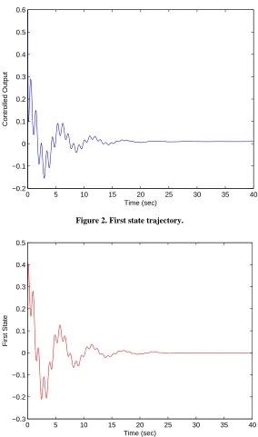
Figure 2. First state trajectory.
0 5 10 15 20 25 30 35 40
−0.3 −0.2 −0.1 0 0.1 0.2 0.3 0.4 0.5
Time (sec)
First State
Figure 3. Second tate trajectory.
Theorem 4.1 yiel e fuzzy state-feedback
con-troller gains of th :
03 9.3657 ,
4 8.8945
8.2863
s
ds th e form
1 2 3
= 0.25,
= 18.54
= 17.723
= 15.7715 K
K
K
The simulation results of the state and controlled- output trajectories are plotted in Figures 1-3. It is quite evident that all the state and output variables of the fuzzy system settle at the equilibrium level within 20 sec.
7. Conclusion
We have addressed the problem of robust
state-feedback controller design for discrete-time Takagi- Sugeno (T-S) fuzzy networked control systems including state quantization. A quantized feedback fuzzy controller has been designed under consideration of effect of net-work-induced delay and data dropout, and the time- varying quantizer has been selected to be logarithmic. By employing a fuzzy Lyapunov-Krasovskii functional, we have derived some LMI-based sufficient conditions for the existence of fuzzy controller. A numerical example
has been given to illustrate the efficiency of the theoretic results.
8. Acknowledgements
The author would like to thank the deanship of scientific research (DSR) at KFUPM for financial support through research group project RG1105-1.
REFERENCES
[1] T. Takagi and M. Sugeno, “Fuzzy Identification of Sys-tems and Its Applications to Modeling and Control,” IEEE Transactions on Systems, Man, and Cybernetics, Vol. 15, No. 1, 1985, pp. 116-132.
[2] K. Tanaka, T. Ikeda and H. Wang, “Robust Stabilization of a Class of Uncertain Nonlinear Systems via Fuzzy Control: Quadratic lizability, Control Theory,
and Linear Matrix Inequalities,” IEEE Transactions on Fuzzy Systems, Vol. 4, No. 1, 1996, pp. 1-13.
doi:10.1109/91.481840 Stabi
] X. Guan and C. Chen, “Delay-Dependent ste
Sy
:10.1109/TFUZZ.2004.825085
[3 Guaranteed
Cost Control for T-S Fuzzy Sy ms with Time Delays,” IEEE Transactions on Fuzzy stems, Vol. 12, No. 2, 2004, pp. 236-249. doi
[4] Y. Cao and P. Frank, “Analysis and Synthesis of Nonlin-ear Time-Delay systems via Fuzzy Control Approach, IEEE Transactions on Fuzzy Systems, Vol. 8, No. 2, 2000 pp. 200- 211. doi:10.1109/91.842153
” , [5] S. Zhou and T. Li, “Robust Stabilization for Delay
Discrete-Time Fuzzy Systems via Basis-Dependent L ed ya- punov-Krasovskii Function,” Fuzzy Sets and Systems, Vol. 151, No. 1, 2005, pp. 139-153.
doi:10.1016/j.fss.2004.08.014
[6] S. Xu and J. Lam, “Robust Control for Uncertain
Delay Fuzzy Systems via Output F ,” IEEE Transactions on Fuzzy Systems
Discrete-Time-back Controllers
eed-, Vol. 13, No. 1, 2005, pp. 82-93.
doi:10.1109/TFUZZ.2004.839661
[7] H. J. Lee, J. B. Park and G. Chen, “Robust Fuzzy Control of Nonlinear Systems with Parametric Uncertainties,” IEEE Transactions on Fuzzy Systems, Vol. 9, No. 2, 2001, pp. 369-379. doi:10.1109/91.919258
[8] S. Chen, W. Chang and S. Su, “Robust Static Output- Feedback Stabilization for Nonlinear Discrete-Time Sys-tems with Time Delay via Fuzzy Control Approach,” Fuzzy Sets and Systems, Vol. 13, No. 2, 2005, pp. 263- 272.
[9] Y. Cao and P. Frank, “Robust Disturbance
Attenua-tion for a Class of Uncertain Discrete-Time Fuzzy Fuzzy Systems, Vol. 8, No. 0.1109/91.868947
Sys-tems,”IEEE Transactions on
4, 2000, pp. 406-415. doi:1
stems, Vol. 36, No. 4, 2006, pp. 954-962.
[11] H. Gao, T. Chen and J. Lam, “A New Delay System Ap-proach to Network-Based Control,” Automatica, Vol. 44, No. 1, 2008, pp. 39-52.
doi:10.1016/j.automatica.2007.04.020
[12] J. Wu and T. Chen, “Design of Networked Control Sys-tems with Packet Dropouts,” IEEE Transactions on Au-tomatic Control, Vol. 52, No. 7, 2007, pp. 1314-1319. [13] A. Zhang and L. Yu, “Output Feedback Stabilization of
Networked Control Systems with Packet Dropouts,” IEEE Transactions on Automatic Control, Vol. 52, No. 9, 2007, pp. 1705-1710. doi:10.1109/TAC.2007.904284 [14] L. Zhang, Y. Shi, T. Chen and B. Huang, “A New
Me-thod for Stabilization of Networked Control Systems with Random Delays,” IEEE Transactions on Automatic Con-trol, Vol. 50, No. 8, 2005, pp. 1177-1181.
[15] M. S. Mahmoud, “Switched Time-Delay Systems,” Sprin- ger-Verlag, New York, 2010.
[16] E. Tian, D. Yue and C. Peng, “Quantized Output Feed-back Control for Networked Control Systems,” Informa-tion Sciences, Vol. 178, 2008, pp. 2734-2749.
/j.ins.2008.01.019
[10] H. Wu, “Delay-dependent Stability Analysis and Stabili-zation for Discrete-Time Fuzzy Systems with State Delay: A Fuzzy Lyapunov-Krasovskii Functional Approach,” IEEE Transactions on Fuzzy Sy
doi:10.1016
Peng and G. Tang, “Guaranteed Cost Control of Linear Systems over Networks with State and Input Quantizations,” IET Control Theory and Application, Vol. 153, No. 6, 20
[17] D. Yue, C.
06, pp. 658-664. doi:10.1049/ip-cta:20050294
[18] P. Chen and C. Yu, “Networked Control of Linear
Systems with State Quantization,” Information Sciences, Vol. 177, 2007, pp. 5763-5774.
doi:10.1016/j.ins.2007.05.025
[19] M. S. Mahmoud, “Delay-Dependent Filtering of a
Class of Switched Discrete-Time State-Delay Systems,” Signal Processing, Vol. 88, No. 11, 2008, pp. 2709-2719. doi:10.1016/j.sigpro.2008.05.014
[20] M. S. Mahmoud, A. W. Saif and P. Shi, “Stabilization of Linear Switched Delay Systems: 2 and 2
Meth-ods,” Journal of Optimization Theory and Applications, Vol. 142, No. 3, 2009, pp. 583-607.
doi:10.1007/s10957-009-9527-2
[21] J. Zhang, Y. Xia and M. S. Mahmoud, “Robust General-ized H2 and Static Output Feedback Control for
Uncertain Discrete-Time Fuzzy Systems,” IET Control Theory and Applications, Vol. 3, No. 7, 2009, pp. 865-876. doi:10.1049/iet-cta.2008.0146
[22] H. Gao, P. Shi and J. Wang, “Parameter-Dependent Ro-bust Stability of Uncertain Time-Delay Systems,” Com-putational & Applied Mathematics, Vol. 206, No. 1, 2007, pp. 366-373. doi:10.1016/j.cam.2006.07.027
[23] H. Gao, J. Lam, C. Wang and Y. Wang, “Delay-Depend- ent Output-Feedback Stabilization of Discrete-Time Sys-tems with Time-Varying State Delay,” IEE Proceedings of Control Theory and Applicatio
2004, pp. 691-698.
ns, Vol. 151, No. 6, ta:20040822
doi:10.1049/ip-c
Copyright © 2012 SciRes. ICA [25] G. Walsh and H. Ye, “Scheduling of Networked Control
Systems,” IEEE Control Systems Magazine, Vol. 21, No. 1, 2001, pp. 57-65. doi:10.1109/37.898792
[26] H. Zhang, D. Yang and T. Chai, “Guaranteed Cost Net-worked Control for T-S Fuzzy Systems with Time
De-ith Time-Variant Delays,”
lays,” Applications and Reviews, Vol. 37, No. 2, 2007, pp. 160-172.
[27] L. Zhang and H. Fang, “Fuzzy Controller Design for
Networked Control System w
Journal of Systems Engineering and Electronics, Vol. 17, No. 1, 2006, pp. 172-176.
doi:10.1016/S1004-4132(06)60030-3