Power Quality Improvement of Large Power System Using a Conventional Method

Power Quality Improvement of Large Power System

Using a Conventional Method

Nazmus Sahadat, Shakhawat Hossain, Arifur Rahman, Sharif Taufique Atique, Md. Touhiduzzaman Department of Electrical and Electronic Engineering, Bangladesh University of Engineering and Technology, Bangladesh

E-mail: [email protected]

Received May 7, 2011; revised May 25, 2011; accepted June 5, 2011

Abstract

Operation of a large power system with maintaining proper power quality is always been a difficult task. It becomes more difficult to maintain the power quality when rapid expansion of previously designed power system occurred. To redesign of such a power system is not feasible and also cost effective. To improve the quality of power of such a large system, conventional methods of compensation can be used. In this paper a power system of 419 buses is analyzed. It is found that 76 buses have under voltage problem. Conventional shunt compensation method is used by connecting capacitor in parallel to the bus. After compensation the system is simulated again and found that the under voltage problem of this large power system is removed. Power factor of the system is also improved.

Keywords:Shunt Compensation, Power Quality, under Voltage, Power Factor, Power Flow, PSAF

1. Introduction

The necessity of energy is increasing day by day. With the development of more sensitive electronic appliances it is mandatory to maintain the quality of power. Many valuable devices can be burnt out due to the cause of low power quality. In the industrial application power quality is most important. Big economical loss can occur due to power quality.

Under voltage problem of large power system is a very common problem. To solve this problem many methods can be used [1-4]. Shunt compensation in the buses is most common method among of them.

In this paper fixed capacitor is used to solve the under voltage problem of a large power system of Bangladesh. Load flow analysis is applied by PSAP of a 419 bus sys-tem before and after connecting fixed capacitor in the low voltage buses. Before connecting of fixed capacitor it is found that 76 buses have under voltage (below 0.9 p.u.). After connecting the fixed capacitor in 45 buses it is found that under voltage problem is totally solved and the power factor of the buses have also improved.

2. Theory of Compensation

Figure 1 shows the simplified model of a power

trans-mission system. Two power grids are connected by a

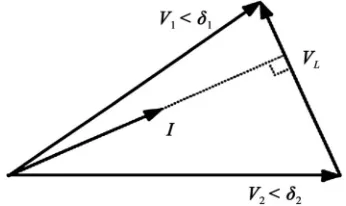
transmission line which is assumed lossless and repre-sented by the reactance XL. V1 < δ1 and V2 <δ2 represent the voltage phasors of the two power grid buses with angle δ = δ1 – δ2 between the two. The corresponding phasor diagram is shown in Figure 2.

The magnitude of the current in the transmission line is given by:





L L L

I V X  V  V  X (1)

Figure 1. Simplified model of power transmission system.

The active and reactive components of the current flow at bus 1 are given by:





1 2sin , 1 1 2cos

d L q L

I V  X I  V V  X (2-3) The active power and reactive power at bus 1 are giv-en by:





1 1 2sin L, 1 1 1 2cos L

P V V  X Q V V V  X (4-5)

Similarly, the active and reactive components of the current flow at bus 2 can be given by:





2 1sin , 2 2 1cos

d L q L

I V  X I  V V  X (6-7)

The active power and reactive power at bus 2 are giv-en by:





2 1 2sin L, 2 2 2 1cos L

P V V  X Q V V V  X (8-9)

Equations (1)-(9) indicate that the active and reactive power/current flow can be regulated by controlling the voltages, phase angles and line impedance of the trans-mission system.

3. Methods of Compensation

The compensation of transmission systems can be di-vided into two main groups: shunt and series compensa-tion [5].

3.1. Series Compensation

Series compensation aims to directly control the overall series line impedance of the transmission line. Tracking back to Equations (1)-(9), the AC power transmission is primarily limited by the series reactive impedance of the transmission line. A series-connected can add a voltage in opposition to the transmission line voltage drop, there- fore reducing the series line impedance [6-8].

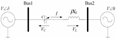
A simplified model of a transmission system with se-ries compensation is shown in Figure 3. The voltage

magnitudes of the two buses are assumed equal as V, and the phase angle between them is δ. The transmission line is assumed lossless and represented by the reactance XL. A controlled capacitor is series-connected in the trans-mission line with voltage addition Vinj. The phase dia-gram is shown in Figure 4.

Figure 3. Simplified transmission system model with series compensation.

Defining the capacitance of C as a portion of the line reactance,

C L

X KX (10) The overall series inductance of the transmission line is,





L C L

X X X  K X (11)

The active power transmitted is,





2 _{1 s}

L

P V K X  in

The reactive power supplied by the capacitor is calcu-lated as:









2 2

2 1 1

C L

Q  V X K K  cos (13)

In Figure 5 shows the power angle curve from which

it can be seen that the transmitted active power increases with K.

3.2. Shunt Compensation

Shunt compensation, especially shunt reactive compen-sation has been widely used in transmission system to regulate the voltage magnitude, improve the voltage quality, and enhance the system stability [9]. Shunt-con-nected reactors are used to reduce the line over-voltages by consuming the reactive power, while shunt-connected capacitors are used to maintain the voltage levels by compensating the reactive power to transmission line.

Figure 4. Phasor diagram of series compensated line volt-ages.

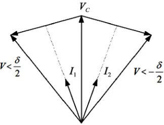
A simplified model of a transmission system with shunt compensation is shown in Figure 6. Figure 7

shows the phasor diagram of corresponding voltages and currents. The voltage magnitudes of the two buses are assumed equal as V, and the phase angle between them is

δ. The transmission line is assumed lossless and repre-sented by the reactance XL At the midpoint of the trans-mission line; a controlled capacitor C is shunt-connected. The voltage magnitude at the connection point is main-tained as V.

As discussed previously, the active powers at bus 1 and bus 2 are equal.



2

1 2 2 L sin

P P  V X   2



As discussed previously, the active powers at bus 1 and bus 2 are equal.

2

4 1 co

2

C L

Q  V X  _ s

 



 (15)

From the power angle curve shown in Figure 8, the

transmitted power can be significantly increased, and the peak point shifts from δ = 90º to δ = 180º. The operation margin and the system stability are increased by the shunt compensation.

The voltage support function of the midpoint com-pensation can easily be extended to the voltage support at the end of the radial transmission, which will be proven by the system simplification analysis. The reactive power compensation at the end of the radial line is especially effective in enhancing voltage stability.

Figure 6. Simplified transmission system model with shunt compensation.

Figure 7. Phasor diagram of shunt compensated line volt-ages and currents.

Figure 8. Power angle curve.

4. Load Flow Analysis

The goal of a power flow study is to obtain complete voltage angle and magnitude information for each bus in a power system for specified load and generator real power and voltage conditions [10]. Once this information is known, real and reactive power flow on each branch as well as generator reactive power output can be analyti-cally determined. Due to the nonlinear nature of this problem, numerical methods are employed to obtain a solution that is within an acceptable tolerance.

The solution to the power flow problem begins with identifying the known and unknown variables in the sys-tem. The known and unknown variables are dependent on the type of bus. A bus without any generators con-nected to it is called a Load Bus. With one exception, a bus with at least one generator connected to it is called a Generator Bus. The exception is one arbitrarily-selected bus that has a generator. This bus is referred to as the Slack Bus.

In the power flow problem, it is assumed that the real power PD and reactive power QD at each Load Bus are known. For this reason, Load Buses are also known as PQ Buses. For Generator Buses, it is assumed that the real power generated PG and the voltage magnitude |V| is known. For the Slack Bus, it is assumed that the voltage magnitude |V| and voltage phase Θ are known. Therefore, for each Load Bus, both the voltage magnitude and angle are unknown and must be solved for; for each Generator Bus, the voltage angle must be solved for; there are no variables that must be solved for the Slack Bus. In a sys-tem with N buses and R generators, there are then 2(N−

1) − (R− 1) unknowns.

In order to solve for the 2(N− 1) − (R− 1) unknowns, there must be 2(N− 1) − (R − 1) equations that do not introduce any new unknown variables. The possible equ-ations to use are power balance equequ-ations, which can be written for real and reactive power for each bus. The real power balance equation is:





1

0  P_i



Pi = Net power injected at bus i.

matrix YBUS corresponding to the ith row and kth column. Bik = Imaginary part of the element in the YBUS corre-sponding to the ith row and kth column

θik = Difference in voltage angle between the ith and kth buses.

The reactive power balance equation is:



1

0  Q_i





Qi = Net reactive power injected at bus i.

Equations included are the real and reactive power balance equations for each Load Bus and the real power balance equation for each Generator Bus. Only the real power balance equation is written for a Generator Bus because the net reactive power injected is not assumed to be known and therefore including the reactive power balance equation would result in an additional unknown variable. For similar reasons, there are no equations written for the Slack Bus.

4.1. Gauss-Seidel Method

This method is based on substituting nodal equations into each other. It is the slower of the two but is the more stable technique. Its convergence is said to be Monotonic. The iteration process can be visualized for two equa-tions:

Although not the best load-flow method, Gauss-Seidel is the easiest to understand and was the most widely used technique until the early 1970s.

4.2. Newton Raphson Method

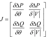
There are several different methods of solving the re-sulting nonlinear system of equations. The most popular is known as the Newton-Raphson Method. This method begins with initial guesses of all unknown variables (voltage magnitude and angles at Load Buses and voltage angles at Generator Buses). Next, a Taylor Series is written, with the higher order terms ignored, for each of the power balance equations included in the system of equations. The result is a linear system of equations that can be expressed as:

1 P J V Q  _       _  _   

  (18) where, ΔP and ΔQ are called the mismatch equations:



1 cos sin

N

i k i k ik ik ik

P P  V V G  B ik



   





1 sin cos

N

i k i k ik ik ik

Q Q _ V V G  B _ik



   



and J is a matrix of partial derivatives known as a Jaco-bean: P P V J Q Q V                          (21)

The linearized system of equations is solved to deter-mine the next guess (m + 1) of voltage magnitude and angles based on:

1

m m

  _ _{  (22)} 1

m m

V  V  V (23)

The process continues until a stopping condition is met. A common stopping condition is to terminate if the norm of the mismatch equations are below a specified tolerance.

5. Simulation and Results

Bangladesh power system is a big system of 419 buses. So the system is divided in to six zones and load flow study is applied in PSAP (Power System Analysis Pro-gram). Newton-Raphson method is used here for solving the load flow problem.

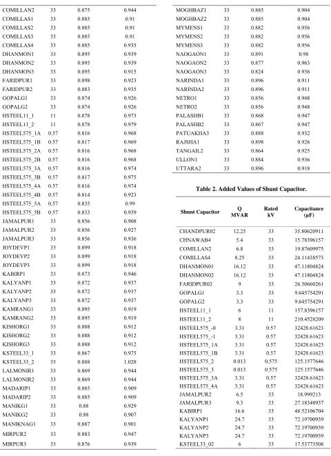
Load flow study is applied on the whole system with-out connecting any compensator. It is found that 76 buses have voltage under 0.9 p.u. To solve this under voltage problem fixed capacitors have installed in 44 buses of them. After adding fixed capacitors, load flow study is applied again and it is found that under voltage problem of whole system has removed. Power factor of the sys-tem has also improved. Table 1 shows the values of bus

voltages in p.u. before and after connecting shunt ca-pacitors.

The added values of shunt capacitors have also been calculated. Table 2 shows the added values of capacitors

in micro Farad.

Table 1. Under Voltage Buses before and after Shunt Com-pensation. BUS ID Rated value (kV) Voltage before compensation [p.u.]

Voltage after shunt compensation

[p.u.]

1204 132 0.893 0.943

CHANDPUR1 33 0.899 0.927

CHANDPUR2 33 0.899 0.946

CHNAWAB1 33 0.888 0.92

CHNAWAB2 33 0.888 0.92

CHNAWAB3 33 0.888 0.92

CHNAWAB4 33 0.87 0.926

COMILLAN2 33 0.875 0.944

COMILLAS1 33 0.885 0.91

COMILLAS2 33 0.885 0.91

COMILLAS3 33 0.885 0.91

COMILLAS4 33 0.885 0.935

DHANMON1 33 0.895 0.939

DHANMON2 33 0.895 0.939

DHANMON3 33 0.895 0.915

FARIDPUR1 33 0.898 0.923

FARIDPUR2 33 0.883 0.935

GOPALG1 33 0.874 0.926

GOPALG2 33 0.874 0.926

HSTEEL11_1 11 0.878 0.973

HSTEEL11_2 11 0.878 0.979

HSTEEL575_1A 0.57 0.816 0.968 HSTEEL575_1B 0.57 0.817 0.969 HSTEEL575_2A 0.57 0.816 0.968 HSTEEL575_2B 0.57 0.816 0.968 HSTEEL575_3A 0.57 0.816 0.974 HSTEEL575_3B 0.57 0.817 0.975 HSTEEL575_4A 0.57 0.816 0.974 HSTEEL575_4B 0.57 0.814 0.923

HSTEEL575_5A 0.57 0.835 0.99

HSTEEL575_5B 0.57 0.833 0.939

JAMALPUR1 33 0.856 0.908

JAMALPUR2 33 0.856 0.927

JAMALPUR3 33 0.856 0.936

JOYDEVP1 33 0.899 0.918

JOYDEVP2 33 0.899 0.918

JOYDEVP3 33 0.899 0.918

KABIRP1 33 0.873 0.946

KALYANP1 33 0.872 0.937

KALYANP2 33 0.872 0.937

KALYANP3 33 0.872 0.937

KAMRANG1 33 0.895 0.919

KAMRANG2 33 0.895 0.919

KISHORG1 33 0.888 0.912

KISHORG2 33 0.888 0.912

KISHORG3 33 0.888 0.912

KSTEEL33_1 33 0.867 0.975

KSTEEL33_2 33 0.888 1.028

LALMONIR1 33 0.869 0.944

LALMONIR2 33 0.869 0.944

MADARIP1 33 0.885 0.909

MADARIP2 33 0.885 0.909

MANIKG1 33 0.88 0.929

MANIKG2 33 0.88 0.907

MANIKNAG1 33 0.887 0.901

MIRPUR2 33 0.883 0.947

MIRPUR3 33 0.876 0.939

MOGHBAZ1 33 0.885 0.904

MOGHBAZ2 33 0.885 0.904

MYMENS1 33 0.882 0.956

MYMENS2 33 0.882 0.956

MYMENS3 33 0.882 0.956

NAOGAON1 33 0.891 0.98

NAOGAON2 33 0.877 0.963

NAOGAON3 33 0.824 0.936

NARINDA1 33 0.896 0.911

NARINDA2 33 0.896 0.911

NETRO1 33 0.856 0.948

NETRO2 33 0.856 0.948

PALASHB1 33 0.868 0.947

PALASHB2 33 0.867 0.947

PATUAKHA3 33 0.888 0.932

RAJSHA1 33 0.898 0.926

TANGAIL2 33 0.864 0.925

ULLON1 33 0.884 0.936

UTTARA2 33 0.896 0.918

Table 2. Added Values of Shunt Capacitor.

Shunt Capacitor Q MVAR

Rated kV

Capacitance (µF)

CHANDPUR02 12.25 33 35.80620911

CHNAWAB4 5.4 33 15.78396157

COMILLAN2 6.8 33 19.87609975

COMILLAS4 8.25 33 24.11438573

DHANMON01 16.12 33 47.11804824 DHANMON02 16.12 33 47.11804824

FARIDPUR02 9 33 26.30660261

GOPALG1 3.3 33 9.645754291

GOPALG2 3.3 33 9.645754291

HSTEEL11_1 6 11 157.8396157

HSTEEL11_2 8 11 210.4528209

HSTEEL575_-0 3.31 0.57 32428.61623 HSTEEL575_-1 3.31 0.57 32428.61623 HSTEEL575_1A 3.31 0.57 32428.61623 HSTEEL575_1B 3.31 0.57 32428.61623 HSTEEL575_2 0.013 0.575 125.1577646 HSTEEL575_3 0.013 0.575 125.1577646 HSTEEL575_3A 3.31 0.57 32428.61623 HSTEEL575_4A 3.31 0.57 32428.61623 JAMALPUR2 6.5 33 18.999213

JAMALPUR3 9.3 33 27.18348937

KABIRP1 16.6 33 48.52106704

KALYANP1 24.7 33 72.19700939

KALYANP2 24.7 33 72.19700939

KALYANP3 24.7 33 72.19700939

KSTEEL33_1 12.25 33 35.80620911

LALMONIR1 5.5 33 16.07625715

LALMONIR2 5.5 33 16.07625715

MANIKG1 10.4 33 30.3987408

MIRPUR2 23.4 33 68.39716679

MIRPUR3 23.4 33 68.39716679

MYMENS1 11 33 32.1525143

MYMENS2 11 33 32.1525143

MYMENS3 11 33 32.1525143

NAOGAON1 12 33 35.07547015

NAOGAON2 12 33 35.07547015

NAOGAON3 12 33 35.07547015

NETRO1 6.5 33 18.999213

NETRO2 6.5 33 18.999213

PALASHB1 5.5 33 16.07625715

PALASHB2 5.5 33 16.07625715

PATUAKHA3 3.5 33 10.23034546

TANGAIL2 11 33 32.1525143

ULLON1 15.6 33 45.5981112

6. Conclusions

The demand of power is increasing enormously day by day. So it has been difficult task to maintain the power quality with the increasing load. As system redesign is much costly so it is necessary to control the parameters of the power system to obtain maximum efficiency.

In this paper such a cost effective shunt compensation method is applied to Bangladesh power system. Here fixed capacitors are used as a shunt compensator to solve the under voltage problem of Bangladesh power system. The under voltage problem is solved successfully and power factor of the system also improved.

7. References

[1] B. M. Zhang and Q. F. Ding, “The Development of

FACTS and Its Control,” Advances in Power System Control, Operation and Management, APSCOM-97. 4th International Conference, Vol. 1, Beijing, 11-14 Novem-ber 1997, pp. 48-53.

[2] J. J. Paserba, “How FACTS Controllers Benefit AC Transmission Systems,” Power Engineering Society Gen-eral Meeting, IEEE, Vol. 2, Warrendale, 10 June 2004, pp. 1257-1262.

[3] A. Edris, “FACTS Technology Development: An Up-date,” Power Engineering Review, IEEE, Vol. 20, No. 3, March 2000, pp. 599-627.

[4] L. Gyugyi, “Application Characteristics of Converter- Based FACTS Controllers,” IEEE Conference on Power System Technology, Vol. 1, Perth, 4-7 December 2000, pp. 391-396.

[5] H. Dag, B. Ozturk and A.Ozyurek, “Application of Series and Shunt Compensation to Turkish National Power Transmission System to Improve System Loadability,”

ELECO’99 Intenational Conference on Electrical and Electronic Engineering, Bursa, 1-5 December 1999, pp. 243-247.

[6] J. R. Daconti and D. C. Lawry, “Increasing Power Trans-fer Capability of Existing Transmission Lines,” Trans-mission and Distribution Conference and Exposition,

IEEE PES, Vol. 3, Schenectady, 7-12 September 2003, pp. 1004-1009.

[7] R. Rajarman, F. Alvarado, A. Maniaci, R. Camfield and S. Jalali, “Determination of Location and Amount of Series Compensation to Increase Power Transfer Capability,”

IEEE Transactions on PowerSystems, Vol. 3, No. 2, 1998, pp. 294-300. doi:10.1109/59.667338

[8] R. S. Naik, K. Vaisakh and K. Anand., “Determination of ATC with PTDF Using Linear Methods in Presence of TCSC,” The 2nd International Conference on Computer and Automation Engineering, Vol. 5, Singapore, 26-28 February 2010, pp. 146-151.

[9] N. G. Hingorani and L. Gyugyi, “Understanding FACTS, Concepts and Technology of Flexible AC Transmission systems,” IEEE Press, New York, 2000.