Efficient Fast Multiplication Free Integer Transformation for the 1 D DCT of the H 265 Standard

Efficient Fast Multiplication Free Integer

Transformation for the 1-D DCT of the H.265

Standard

Mohamed Nasr Haggag1_{, Mohamed El-Sharkawy}2_{, Gamal Fahmy}3_{, Maher Rizkalla}1

1_{German University at CairoNew Cairo City, Cairo, Egypt;} 2_{Egypt Japan University of Science and Technology Borg Al Arab,} Alexandria, Egypt; 3_{Electrical Engineering Department, Assiut University, Assiut, Egypt.}

Email: [email protected]

Received January 21st _{2010; revised June 30}th _{2010; accepted July 5}th _2010.

ABSTRACT

In this paper, efficient one-dimensional (1-D) fast integer transform algorithms of the DCT matrix for the H.265 stan-dard is proposed. Based on the symmetric property of the integer transform matrix and the matrix operations, which denote the row/column permutations and the matrix decompositions, along with using the dyadic symmetry modification on the standard matrix, the efficient fast 1-D integer transform algorithms are developed. Therefore, the computational complexities of the proposed fast integer transform are smaller than those of the direct method. In addition to computa-tional complexity reduction one of the proposed algorithms provides transformation quality improvement, while the other provides more computational complexity reduction while maintaining almost the same transformation quality. With lower complexity and better transformation quality, the first proposed fast algorithm is suitable to accelerate the quality-demanding video coding computations. On the other hand, with the significant lower complexity, the second proposed fast algorithm is suitable to accelerate the video coding computations.

Keywords: Fast Algorithm, HDTV, H.265, ICT, Order-16 Transform, Video Coding

1. Introduction

NOWDAYS the demand for higher quality digital video products and faster digital video applications in our daily life activities is increasing. These demands start from our daily necessary needs, like video conferencing, television and surveillance, up to our entertainment, iPods, internet video streaming, digital cameras, and all high definition (HD) products [1,2]. There have been two primary stan-dards organizations driving the definition of video coding. The International Telecommunications Union (ITU), which is an organization focused on telecommunication applications and has created the series of H.26x standards for low bit rate video telephony. These include H.261, H.262, H.263 and H.264. The other organization is the International Standards Organization (ISO), which is more focused on consumer applications and has defined the MPEG series standards for compressing moving pic-tures. The MPEG standard series include MPEG-1, MPEG-2 and MPEG-4 [1,2].

In [3], the 16 × 16 2-D matrix for the H.265 standard DCT is revealed, using the decomposition and the

mod-ification techniques used in [4-7], this paper will intro-duce two proposed algorithm that will aim to reintro-duce the complexity of the algorithm implementation in addition to making it multiplication-free.

The rest of this paper is organized as follows. In Sec-tion 2, review of the integer transformaSec-tion for the H.265 standard is described. In Section 3, the two proposed efficient fast integer transform algorithms for the 2-D H.265 standard are introduced with the proposed matrix factorizations. Then the computational complexities of these proposed algorithms are discussed. In Section 4, analysis and comparison of transformation quality be-tween the proposed fast algorithms and the original me-thod is shown. In Section 5, comparison of computation-al complexity done in Section 3 and qucomputation-ality evcomputation-aluation done in Section 4 is discussed. Finally, we give a conclu-sion.

2. Review of the Integer Transformation for

the H.265 Standard

high definition video processing. From [3], the matrix of the 2-D 16 × 16 integer cosine transformation for the H.265 standard is shown in Equation (1).

The matrix elements in Equation (1) shows that there is

symmetric properties between the left side and right side of the matrix, this property will be exploited using matrix decomposition in order to this matrix into the product of sparse matrices in the next section.

𝑇𝑇 =

⎣ ⎢ ⎢ ⎢ ⎢ ⎢ ⎢ ⎢ ⎢ ⎢ ⎢ ⎢ ⎢ ⎢ ⎢

⎡₄₅32 32₄₃ 32_{40 35}32 ₂₉32 ₂₁32 32₁₃ 32_{4 −}32_{4 −}32_{13 −}32_{21 −}32_{29 −}32_{35 −}32_{40 −}32_{43 −}32₄₅

44 38 25 9 −9 −25 −38 −44 −44 −38 −25 −9 9 25 38 44 43 29 4 −21 −40 −45 −35 −13 13 35 45 40 21 −4 −29 −43 42 17 −17 −42 −42 −17 17 42 42 17 −17 −42 −42 −17 17 42 40 4 −35 −43 −13 29 45 21 −21 −45 −29 13 43 35 −4 −40 38 −9 −44 −25 25 44 9 −38 −38 9 44 25 −25 −44 −9 38 35 −21 −43 4 45 13 −40 −29 29 40 −13 −45 −4 43 21 −35 32 −32 −32 32 32 −32 −32 32 32 −32 −32 32 32 −32 −32 32 29 −40 −13 45 −4 −43 21 35 −35 −21 43 4 −45 13 40 −29 25 −44 9 38 −38 −9 44 −25 −25 44 −9 −38 38 9 −44 25 21 −45 29 13 −43 35 4 −40 40 −4 −35 43 −13 −29 45 −21 17 −42 42 −17 −17 42 −42 17 17 −42 42 −17 −17 42 −42 17 13 −35 45 −40 21 4 −29 43 −43 29 −4 −21 40 −45 35 −13

9 −25 38 −44 44 −38 25 −9 −9 25 −38 44 −44 38 −25 9 4 −13 21 −29 35 −40 43 −45 45 −43 40 −35 29 −21 13 −4⎦⎥

⎥ ⎥ ⎥ ⎥ ⎥ ⎥ ⎥ ⎥ ⎥ ⎥ ⎥ ⎥ ⎥ ⎤

(1)

3. Proposed Algorithms

In this section, two proposed algorithm for efficient fast multiplication-free for the H.265 standard are presented. The proposed algorithms are done using a combination of Modified Integer Cosine Transformation, matrix de-composition and dyadic symmetry. The common part in the complexity reduction is discussed first, then each algorithm is presented individually and its complexity is calculated with it. The aim of the proposed algorithms is to reduce the computational complexities, which are refe-

rred to as the numbers of additions and shift operations as much as possiblewhile maintaining reasonable error margin. The DCT matrix for the H.265 is given as T in Equation (1).

The symmetric property of the transformation matrix is exploited to decompose it into the product of two sparse matrices. so the transformation matrix in Equation 1 can be rewritten in Equation (2) [4,7].

1

T

T T P= ⋅ (2)

𝑇𝑇𝑇𝑇 =

⎣ ⎢ ⎢ ⎢ ⎢ ⎢ ⎢ ⎢ ⎢ ⎢ ⎢ ⎢ ⎢ ⎢ ⎢

⎡32₀ 32₀ 32₀ 32₀ 32₀ 32₀ 32₀ 32_{0 −}0_{4 −}0_{13 −}0_{21 −}0_{29 −}0_{35 −}0_{40 −}0_{43 −}0₄₅

44 38 25 9 −9 −25 −38 −44 0 0 0 0 0 0 0 0 0 0 0 0 0 0 0 0 13 35 45 40 21 −4 −29 −43 42 17 −17 −42 −42 −17 17 42 0 0 0 0 0 0 0 0

0 0 0 0 0 0 0 0 −21 −45 −29 13 43 35 −4 −40 38 −9 −44 −25 25 44 9 −38 0 0 0 0 0 0 0 0

0 0 0 0 0 0 0 0 29 40 −13 −45 −4 43 21 −35 32 −32 −32 32 32 −32 −32 32 0 0 0 0 0 0 0 0

0 0 0 0 0 0 0 0 −35 −21 43 4 −45 13 40 −29 25 −44 9 38 −38 −9 44 −25 0 0 0 0 0 0 0 0

0 0 0 0 0 0 0 0 40 −4 −35 43 −13 −29 45 −21 17 −42 42 −17 −17 42 −42 17 0 0 0 0 0 0 0 0

0 0 0 0 0 0 0 0 −43 29 −4 −21 40 −45 35 −13 9 −25 38 −44 44 −38 25 −9 0 0 0 0 0 0 0 0 0 0 0 0 0 0 0 0 45 −43 40 −35 29 −21 13 −4⎦⎥

𝑃𝑃1=

⎣ ⎢ ⎢ ⎢ ⎢ ⎢ ⎢ ⎢ ⎢ ⎢ ⎢ ⎢ ⎢ ⎢ ⎢

⎡ 1₀ 0₁ 0_{0 0}0 0₀ 0_{0 0}0 ₀0 0 0 0 0 0 0 0 1_{0 0 0 0 0 0 1 0}

0 0 1 0 0 0 0 0 0 0 0 0 0 1 0 0 0 0 0 1 0 0 0 0 0 0 0 0 1 0 0 0 0 0 0 0 1 0 0 0 0 0 0 1 0 0 0 0 0 0 0 0 0 1 0 0 0 0 1 0 0 0 0 0 0 0 0 0 0 0 1 0 0 1 0 0 0 0 0 0 0 0 0 0 0 0 0 1 1 0 0 0 0 0 0 0 0 0 0 0 0 0 0 −1 1 0 0 0 0 0 0 0 0 0 0 0 0 0 −1 0 0 1 0 0 0 0 0 0 0 0 0 0 0 −1 0 0 0 0 1 0 0 0 0 0 0 0 0 0 −1 0 0 0 0 0 0 1 0 0 0 0 0 0 0 −1 0 0 0 0 0 0 0 0 1 0 0 0 0 0 −1 0 0 0 0 0 0 0 0 0 0 1 0 0 0 −1 0 0 0 0 0 0 0 0 0 0 0 0 1 0

−1 0 0 0 0 0 0 0 0 0 0 0 0 0 0 1⎦⎥

⎥ ⎥ ⎥ ⎥ ⎥ ⎥ ⎥ ⎥ ⎥ ⎥ ⎥ ⎥ ⎥ ⎤

Where

T r r

T =P T⋅ (3)

𝑃𝑃𝑃𝑃=

⎣ ⎢ ⎢ ⎢ ⎢ ⎢ ⎢ ⎢ ⎢ ⎢ ⎢ ⎢ ⎢ ⎢ ⎢

⎡1 0 0 0 0 0 0 0 0 0 0 0 0 0 0 0_{0 0 0 0 0 0 0 0 1 0 0 0 0 0 0 0}

0 1 0 0 0 0 0 0 0 0 0 0 0 0 0 0 0 0 0 0 0 0 0 0 0 1 0 0 0 0 0 0 0 0 1 0 0 0 0 0 0 0 0 0 0 0 0 0 0 0 0 0 0 0 0 0 0 0 1 0 0 0 0 0 0 0 0 1 0 0 0 0 0 0 0 0 0 0 0 0 0 0 0 0 0 0 0 0 0 0 0 1 0 0 0 0 0 0 0 0 1 0 0 0 0 0 0 0 0 0 0 0 0 0 0 0 0 0 0 0 0 0 0 0 1 0 0 0 0 0 0 0 0 1 0 0 0 0 0 0 0 0 0 0 0 0 0 0 0 0 0 0 0 0 0 0 0 1 0 0 0 0 0 0 0 0 1 0 0 0 0 0 0 0 0 0 0 0 0 0 0 0 0 0 0 0 0 0 0 0 1 0 0 0 0 0 0 0 0 1 0 0 0 0 0 0 0 0 0 0 0 0 0 0 0 0 0 0 0 0 0 0 0 1⎦⎥

⎥ ⎥ ⎥ ⎥ ⎥ ⎥ ⎥ ⎥ ⎥ ⎥ ⎥ ⎥ ⎥ ⎤

and

𝑇𝑇𝑃𝑃 =

⎣ ⎢ ⎢ ⎢ ⎢ ⎢ ⎢ ⎢ ⎢ ⎢ ⎢ ⎢ ⎢ ⎢ ⎢

⎡₄₄32 ₃₈32 ₂₅32 32_{9 −}32_{9 −}32_{25 −}32_{38 −}32_{44 0}0 0₀ 0₀ 0₀ 0₀ 0₀ 0₀ 0₀

42 17 −17 −42 −42 −17 17 42 0 0 0 0 0 0 0 0 38 −9 −44 −25 25 44 9 −38 0 0 0 0 0 0 0 0 32 −32 −32 32 32 −32 −32 32 0 0 0 0 0 0 0 0 25 −44 9 38 −38 −9 44 −25 0 0 0 0 0 0 0 0 17 −42 42 −17 −17 42 −42 17 0 0 0 0 0 0 0 0 9 −25 38 −44 44 −38 25 −9 0 0 0 0 0 0 0 0 0 0 0 0 0 0 0 0 −4 −13 −21 −29 −35 −40 −43 −45 0 0 0 0 0 0 0 0 13 35 45 40 21 −4 −29 −43 0 0 0 0 0 0 0 0 −21 −45 −29 13 43 35 −4 −40 0 0 0 0 0 0 0 0 29 40 −13 −45 −4 43 21 −35 0 0 0 0 0 0 0 0 −35 −21 43 4 −45 13 40 −29 0 0 0 0 0 0 0 0 40 −4 −35 43 −13 −29 45 −21 0 0 0 0 0 0 0 0 −43 29 −4 −21 40 −45 35 −13 0 0 0 0 0 0 0 0 45 −43 40 −35 29 −21 13 −4⎦⎥

The function of P1 is the post-process matrix for the

input data to the matrix multiplication, and the post- process only uses the additions and subtracts. The com-putational complexities of P1 are 16 additions. In

Equa-tion (2), the elements of TT are scattered; the

rearrange-ment of the elerearrange-ments in TT is required to group the

ele-ments of TT into two 8 × 8 independent matrices. Pr is a

pre-process matrix that permutes the rows of T, so that it is rewritten as in Equation (3) [4,7].

As shown in Equation (3), the matrix Pr can be used as

a pre-process matrix. Pr doesn’t have any complexity at

all while serving the purpose of rearranging TT into Tr

where the matrix can be easily represented as the direct sum of its two non-zero areas. The result of the direct sum is shown in Equation (4).

00 11

r

T =T ⊕T (4) Where

00

32 32 32 32 32 32 32 32

44 38 25 9 9 25 38 44

42 17 17 42 42 17 17 42

38 9 44 25 25 44 9 38

32 32 32 32 32 32 32 32

25 44 9 38 38 9 44 25

17 42 42 17 17 42 42 17

9 25 38 44 44 38 25 9

T    _{− − − −}     − − − −   _{− − − −}    =  _{− − − −}    − − − −    _{− − − −}    − − − −     And 11

4 13 21 29 35 40 43 45

13 35 45 40 21 4 29 43

21 45 29 13 43 35 4 40

29 40 13 45 4 43 21 35

35 21 43 4 45 13 40 29

40 4 35 43 13 29 45 21

43 29 4 21 40 45 35 13

45 43 40 35 29 21 13 4

T − − − − − − − −    _{− − −}    − − − − −   _{− − −}    = _{− − − −}    − − − − −   _{− − − − −}    − − − −    

The computation of T00 can be called the computation

of the even frequency part in the transform matrix, and the computation of T11 can be called the computation of

the odd frequency part in the transform matrix [4]. In Equation (4), the integers of matrix T00 have the

symmetry property, using matrix decomposition T00 can

be expressed as the product of the three sparse matrices R1, T0 and R2 as was done with the original matrix T

[4,7]. The result of the decomposition for T00 is shown in Equation (5).

00 r 0 1

T =R T R⋅ ⋅ (5)

Where

1 0 0 0 0 0 0 0 0 0 0 0 1 0 0 0 0 1 0 0 0 0 0 0 0 0 0 0 0 1 0 0 0 0 1 0 0 0 0 0 0 0 0 0 0 0 1 0 0 0 0 1 0 0 0 0 0 0 0 0 0 0 0 1

r R             =               0

32 32 32 32 0 0 0 0

42 17 17 42 0 0 0 0

32 32 32 32 0 0 0 0

17 42 42 17 0 0 0 0

0 0 0 0 9 25 38 44

0 0 0 0 25 44 9 38

0 0 0 0 38 9 44 25

0 0 0 0 44 38 25 9

T    _{− −}     − −   _{− −}    =  _{− − − −}    −    _{− − −}    − −     And 1

1 0 0 0 0 0 0 1 0 1 0 0 0 0 1 0 0 0 1 0 0 1 0 0 0 0 0 1 1 0 0 0 0 0 0 1 1 0 0 0 0 0 1 0 0 1 0 0 0 1 0 0 0 0 1 0 1 0 0 0 0 0 0 1 R             =  ₋    −    ₋    −    

As shown in the above equation, R1 can be implemented

using additions and subtractions only and have a com-plexity of 8 additions, while Rr doesn’t have any

com-plexity at all [4], as for T0 it can be expressed by the

di-rect sum of matrices T0Eand T0O, as shown in Equation

(6).

0 0E 0O

T =T ⊕T (6) Where

0

32 32 32 32

42 17 17 42

32 32 32 32

17 42 42 17

E T    _{− −}    =  − −   _{− −}    0

9 25 38 44

25 44 9 38

38 9 44 25

44 38 25 9

O T − − − −    ₋    = − − −   _{− −}   

The symmetry of the matrix T0E can be further exploited

the product of sparse matrices U1 and U2 [4], as shown in

Equation (7).

0E 1 2

T =U U⋅ (7) Where

1

32 32 0 0

0 0 17 42

32 32 0 0

0 0 42 17

U    _{− −}    =  −   ₋    And 2

1 0 0 1

0 1 1 0

0 1 1 0

1 0 0 1 U       =  −  ₋   

In Equation (7), U2 can be implemented using

addi-tions and subtracaddi-tions only and have a complexity of 4 additions, while U1 can be implemented using 10

addi-tions and 10 shifts. This would sum up to a complexity of 14 addition and 10 shift operations for Equation (7) [4].

Although there is no symmetry present in matrix T0O,

the matrix addition can be used to segment the matrix into two matrices with more value coherence in their elements, as shown in Equation (8).

0O 0 1

T =K +K (8)

Where ₀

9 24 40 36

24 36 9 40

40 9 36 24

36 40 24 9

K − − − −    ₋    = − − −   _{− −}   

And ₁

0 1 2 8

1 8 0 2

2 0 8 1

8 2 1 0 K − −       =  −     

After using the matrix addition, K0 can be simplified

using matrix decomposition into the product of matrices K2 and K3. The result of the decomposition for K0 is

shown in Equation (9).

0 2 3

K =K K⋅ (9) Where

2

1 0 0 4 0 1 4 0

0 4 1 0

4 0 0 1 K       =  −  ₋    And 3

9 8 8 0

8 0 9 8

8 9 0 8

0 8 8 9

K − −   _{− −}    =  −    − − −  

As shown in the above equation; K1 can be implement-

ted using additions and shifts only and have a complexity of 8 additions and 8 shifts, the addition between K1 and

the product of K2 and K3 has a complexity of 4 additions,

As for the matrix K2 it have a complexity of 4 additions

and 4 shifts, while on the other hand K3 have a

complex-ity of 12 additions and 4 shifts. This in the end sums the complexity of T0O to 28 additions and 16 shifts [4,5]. All

of the above decomposition and summation sum the complexity of T00 to 66 additions and 32 shifts [4,5].

Turning to matrix T11 which represents the computa-tion of the odd frequency part, the matrix as shown in Equation (10), doesn't have the symmetric property within its elements, in order to be able to decompose this matrix the modification techniques will be used. For the decomposition of this matrix two proposed algorithms will be presented in this paper.

3.1 Proposed Algorithm 1

For Proposed Algorithm 1, the odd frequency modified integer cosine transformation matrix based on the dyadic symmetry concept used by Wai-Kuen Cham in [7] is obtained by modifying the positions of the elements in the matrix to provide the matrix basic vectors with or-thogonality regardless of the matrix elements values [7]. The matrix T11 and the modified matrix are shown in Equation (10) below.

11 1mod

T∶=T ₍₁₀₎

Where

11

4 13 21 29 35 40 43 45

13 35 45 40 21 4 29 43

21 45 29 13 43 35 4 40

29 40 13 45 4 43 21 35

35 21 43 4 45 13 40 29

40 4 35 43 13 29 45 21

43 29 4 21 40 45 35 13

45 43 40 35 29 21 13 4

T − − − − − − − −    _{− − −}    − − − − −   _{− − −}    = _{− − − −}    − − − − −   _{− − − − −}    − − − −     and 1mod

4 13 21 29 35 40 43 45

35 40 43 45 4 13 21 29

21 29 4 13 43 45 35 40

45 43 40 35 29 21 13 4

43 45 35 40 21 29 4 13

13 4 29 21 40 35 45 43

29 21 13 4 45 43 40 35

40 35 45 43 13 4 29 21

T − − − − − − − −    _{− − − −}    − − − −   _{− − − −}    = _{− − − − −}    − − − −   _{− − − −}    − − − −    

Replacing T11 with T1mod as the new odd frequency

elements as was done in the matrix T00O, as shown in

Equation (11).

1mod m1 m2

T =T +T (11) Where

1

4 16 24 32 36 44 44 44

36 44 44 44 4 16 24 32

24 32 4 16 44 44 36 44

44 44 44 36 32 24 16 4

44 44 36 44 24 32 4 16

16 4 32 24 44 36 44 44

32 24 16 4 44 44 44 36

44 36 44 44 16 4 32 24

m T − − − − − − − −    _{− − − −}    − − − −    − − − −   = _{− − − − −}    − − − −   _{− − − −}    − − − −    

and 2

0 3 3 3 1 4 1 1

1 4 1 1 0 3 3 3

3 3 0 3 1 1 1 4

1 1 4 1 3 3 3 0

1 1 1 4 3 3 0 3

3 0 3 3 4 1 1 1

3 3 3 0 1 1 4 1

4 1 1 1 3 0 3 3

m T −   _{− − −}     − −   _{− − −}    =  _{− −}    − − −    _{− −}    − − −    

In Equation (11), the segment Tm1 from the matrix

ad-dition segmentation done on the matrix T1mod has

sym-metric properties; hence it can be further simplified using matrix decomposition algorithm into the product of three sparse matrices [7]. The result of this matrix decomposi-tion is shown in Equadecomposi-tion (12).

1 1 2 3 4

m

T =M M M⋅ ⋅ ⋅ (12)

Where 1

2 0 1 1 1 3 1 0

3 1 1 1 0 2 0 1

1 3 1 0 1 0 2 1

0 1 0 1 3 1 1 2

1 1 3 2 0 1 0 1

1 1 1 0 2 0 1 3

0 2 0 1 1 1 3 1

1 0 2 3 1 1 1 0

M − − − −    ₋    − − −   _{− −}    =  _{− − − −}    − −    _{− − − − −}    − − −     2

0 0 0 0 1 1 0 1

0 0 1 1 0 0 1 0

0 1 0 1 0 0 1 0

0 1 1 0 0 0 1 0

0 1 1 1 0 0 0 0

1 0 0 0 0 1 0 1

1 0 0 0 1 0 0 1

1 0 0 0 1 1 0 0

M −        − −   _{− −}    =  _{− −}    − − −   _{− −}    −     and 3

1 1 2 0 1 0 2 0

2 0 1 1 2 0 1 0

2 1 0 0 1 1 2 0

1 1 0 2 0 1 0 2

0 2 1 1 0 2 0 1

1 2 0 0 1 1 0 2

0 0 2 1 2 0 1 1

0 0 1 2 0 2 1 1

M − −   _{− − −}     − − −    −   =  ₋    − − −    _{− − −}       

As shown from the equation above; M1 can be

imple-mented using additions and shifts only and have a com-plexity of 48 additions and 8 shifts, while M2 can be

im-plemented using only additions and have a complexity of 16 additions, As for the matrix M3 it have a complexity

of 32 additions and 8 shifts. This in the end sums the complexity of Tm1 to 96 additions and 40 shifts [7]. On

the other hand, Tm2 can be implemented using additions

and shifts only, and has a complexity of 72 additions and 8 shifts [4,5,7].

By using equations from Equation (2) to Equation (12), the efficient fast multiplication-free integer transforma-tion for the 2-D DCT matrix for the H.265 standard for proposed algorithm 1 is given as shown in Equation (13).

(

)

(

(

)

)

{

.

r r

T P= _R ⋅_U U⋅ ⊕ K + K K⋅ _⋅R_⊕

(

)

}

1 1 2 3 4 1

m

T M M M P

 + ⋅ ⋅ ⋅  ⋅

  (13)

3.2 Proposed Algorithm 2

In the proposed algorithm presented in this section the same complexity reduction and decomposition tech-niques will be done, the difference will be that in the odd frequencies matrix in the step done in Equation (10) in-stead of only using dyadic symmetry to rearrange the elements of the matrix, a modification in values of the elements will be done so that it matches the matrix Tm1 in Equation (11). The resultant odd frequency matrix is given in Equation (14).

11 1mod 2

T∶=T (14)

Where

1mod 2

4 16 24 32 36 44 44 44

36 44 44 44 4 16 24 32

24 32 4 16 44 44 36 44

44 44 44 36 32 24 16 4

44 44 36 44 24 32 4 16

16 4 32 24 44 36 44 44

32 24 16 4 44 44 44 36

44 36 44 44 16 4 32 24

T − − − − − − − −    _{− − − −}    − − − −   _{− − − −}    = _{− − − − −}    − − − −   _{− − − −}    − − − −    

The odd frequency matrix for proposed algorithm 2

the same manner as done in Equation (12) in Subsection 3.1. This means that the two proposed algorithm have exactly the same decomposition and segmentation, the only exception is that the odd frequency part for proposed algorithm 2 consists of Tm1 only while for proposed

algo-rithm 1 it consists of the addition of Tm1 and Tm2.

By using equations from Equation (2) to Equation (14), the efficient fast multiplication-free integer transforma-tion for the 2-D DCT matrix for the H.265 standard for proposed algorithm 2 is given as shown in Equation (15).

(

)

(

(

)

)

{

r r

T P= ⋅ _R ⋅_U U⋅ ⊕ K + K K⋅ _⋅R_⊕

(

)

}

 ⋅ ⋅ ⋅  ⋅

  (15)

For the proposed algorithms and the original algorithm, the complexity evaluation is done by calculating the number of additions, shifts and multiplications needed to implement it. The complexity evaluation summary for the proposed and original algorithms is shown in Table 1.

4. Analysis and Comparison of

Transformation Quality

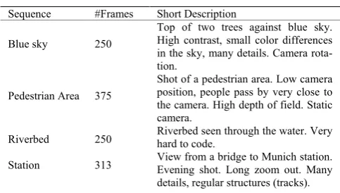
In order to test the efficiency of the proposed algorithms, evaluation of the quality of the reconstructed video com-pared to the original video is done using the quality as-sessment metrics; the three quality metrics used in this paper are the MSE, PSNR and the SSIM. The tests done in this section are applied to standard high definition video quality assessment sequences as developed by Dr. Karl Mauthe at Taurus Media Technik. The full descrip-tion of the test sequences used is shown in Table 2.

Using the Matlab computational tool the quality me-trics for original and the proposed algorithms were cal-culated for 100 frames of the four different standard test sequences. The aim is to evaluate the algorithms quality and reliability, and determine the efficiency of each of the proposed algorithms compared to the original.

Table 1. Complexity Evaluation Comparison table for Origi- nal and Proposed Algorithms

Complexity Operation Original

Algorithm Proposed Algo-rithm 1 Proposed Al-gorithm 2

Additions 240 242 162

Multiplications 256 0 0

Shifts 0 58 50

Table 2. Test Sequences Information

Sequence #Frames Short Description

Blue sky 250

Top of two trees against blue sky. High contrast, small color differences in the sky, many details. Camera rota-tion.

Pedestrian Area 375

Shot of a pedestrian area. Low camera position, people pass by very close to the camera. High depth of field. Static camera.

Riverbed 250 Riverbed seen through the water. Very _{hard to code.}

Station 313 View from a bridge to Munich station. _{Evening shot. Long zoom out. Many} details, regular structures (tracks).

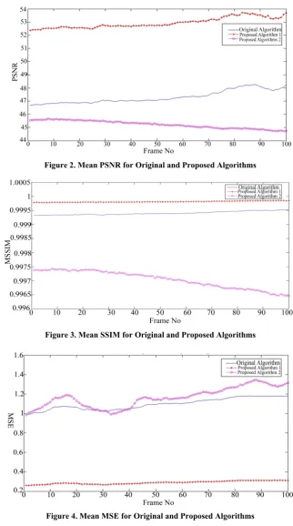
The quality metrics results of the quality assessment for the Blue Sky sequence are shown in the Figures 1, 2

and 3.

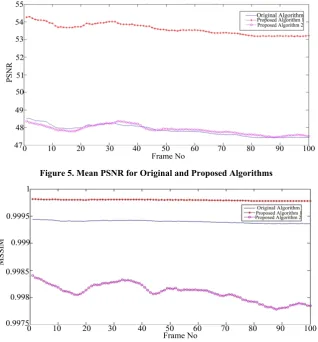
The quality metrics results of the quality assessment for the Pedestrian Area sequence are shown in the Fig-ures 4, 5 and 6.

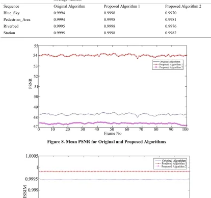
The quality metrics results of the quality assessment for the Riverbed sequence are shown in the Figures 7, 8

and 9.

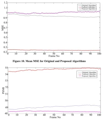
The quality metrics results of the quality assessment for the Station_2 sequence are shown in the Figures 10,

11 and 12.

The figures from 1 to 12 show all the test results done to evaluate the quality of the proposed algorithms com-pared to the original algorithm, all these results are

Figure 2. Mean PSNR for Original and Proposed Algorithms

Figure 3. Mean SSIM for Original and Proposed Algorithms

Figure 4. Mean MSE for Original and Proposed Algorithms

summarized and combined with the complexity of all the algorithms to determine the efficiency of the pro-posed algorithms. Tables 3, 4 and 5 show the summa-rized results for the MSE, PSNR and the MSSIM re-spectively.

5. Comparison of Computational

Complexity and Quality Evaluation

Figure 5. Mean PSNR for Original and Proposed Algorithms

Figure 6. Mean SSIM for Original and Proposed Algorithms

Figure 7. Mean MSE for Original and Proposed Algorithms

Table 3. Average MSE Comparison table for Original and Proposed Algorithms

Average MSE

Sequence Original Algorithm Proposed Algorithm 1 Proposed Algorithm 2

Blue_Sky 1.2513 0.3399 2.8050

Pedestrian_Area 1.0966 0.2893 1.1636

Riverbed 1.0009 0.2646 1.4918

Table 4. Average PSNR Comparison table for Original and Proposed Algorithms

Average PSNR

Sequence Original Algorithm Proposed Algorithm 1 Proposed Algorithm 2

Blue_Sky 47.3093 52.9384 45.2233

Pedestrian_Area 47.8787 53.5946 47.8456

Riverbed 48.2731 54.0194 47.3802

Station 49.0446 54.7329 48.3484

Table 5. Average SSIM Comparison table for Original and Proposed Algorithms

Average MSSIM

Sequence Original Algorithm Proposed Algorithm 1 Proposed Algorithm 2

Blue_Sky 0.9994 0.9998 0.9970

Pedestrian_Area 0.9994 0.9998 0.9981

Riverbed 0.9995 0.9998 0.9976

Station 0.9995 0.9998 0.9982

Figure 8. Mean PSNR for Original and Proposed Algorithms

Figure 10. Mean MSE for Original and Proposed Algorithms

Figure 11. Mean PSNR for Original and Proposed Algorithms

between the results of Section 3 and Section 4.

In terms of quality assessment Table 3 clearly shows the advantage of Proposed Algorithm 1 over Proposed Algorithm 2 and even the Original algorithm as it was able to achieve the smallest values for the MSE index over 4 different test sequences. Table 4 backs the results shown in Table 3, and also shows that the different in quality measured by the PSNR index between the ori-ginnal algorithm and Proposed Algorithm 2 is not high, which means that both achieve comparable qualities.

Table 5 shows that according to a more (HVS) based index, Proposed Algorithm 1 still achieve the best result with the original algorithm coming in second place, and proposed algorithm achieving lower structural similarity than both. However the values in this table indicate that the results for the three algorithms are all almost in the same range, and achieve what is considered high struc-tural similarity. These improved results achieved by the proposed algorithms compared to the original one are due to applying the dyadic symmetry on the transforma-tion matrix odd-frequency part which makes the trans-formation matrix as a whole symmetric and hence elimi-nates the transformation error as the product of the transformation matrix multiplied by its transpose will yield an identity matrix.

As for the complexity point of view, taking into con-sideration that multiplications are the process in terms of complexity and hardware followed by additions and fi-nally shifts. Table 1 clearly shows the superiority of proposed Algorithm 2 over the other two algorithms in terms of less complexity, and emphasis the fact that both of the proposed algorithms are multiplication-free, also the table shows that proposed Algorithm 1 is far less complex than the original algorithm, although it requires two more additions than the original algorithm, it has no multiplications and small number of shifts.

Finally form all the results obtained in this section, it can be concluded that the proposed Algorithm 1 achieves the highest quality in encoding and decoding while main-taining less complexity than the original algorithm, which means that it would be suitable for quality-oriented appli-cations, however on the other hand proposed Algorithm 2 achieves the dramatically less complexity than the origi-nal algorithm without having any noticeable or detectable quality degradation, which makes this algorithm suitable for speed or hardware oriented applications.

6. Conclusions

A new 16 × 16 DCT matrix was recently introduced for the highly anticipated H.265 standard, this DCT matrix is

developed for high definition videos encoding and de-coding, the aim is to make them less complex and faster for video communication and transmission, like in high definition broadcasting and storage. Two new algorithms were proposed in this paper. The first technique is a quality oriented algorithm while offering multiplica-tion-free complexity. The second algorithm is a com-plexity and speed oriented algorithm while maintaining almost the same quality offered by the original algorithm.

The aim of proposing an efficient fast 1-D algorithm for this DCT matrix is to reduce the complexity and hence the hardware and increase the speed of computa-tion to meet the constantly improving demands in the fields of communication and transmission. Quality As-sessment Tests were carried out and the quality metrics MSE, PSNR and SSIM were calculated to evaluate the performance of the proposed algorithms compared to the original one. The test results showed that the first pro-posed algorithm offers better quality, objective and sub-jective, while offering less complexity and multiplica-tion-free computation. While the second proposed algo-rithm offers almost the same quality, objective and sub-jective, while offering much less complexity and multip-lication-free computation than the original algorithm and the first proposed one.

REFERENCES

[1] J.-B. Lee and H. Kalva, “The VC-1 and H.264 Video Compression Standards for Broadband Video Services,” Springer, New York, 2008.

[2] H. 264/MPEG-4 Part 10: Overview. http://www.vcodex. com/files/h264_overview_orig.pdf

[3] http://www.h265.net/index.php?s=dct

[4] C.-P. Fan and G.-A. Su, “Efficient Fast 1-D 8×8 Inverse Integer Transform for VC-1 Application,” IEEE Transac-tions on Circuits and Systems for Video Technology, Vol. 19, No. 4, 2009, pp. 584-590.

[5] C.-P. Fanm and G.-A. Su, “Efficient Low-Cost Sharing Design of Fast 1-D Inverse Integer Transform Algorithms for H.264/AVC and VC-1,” IEEE Signal Processing Let-ters, Vol. 15, 2008, pp. 926-929.

[6] W.-K. Cham, “Development of Integer Cosine Transfor-mation by the Principle of Dyadic Symmetry,” IEEE Proceedings, Vol. 136, No. 4, August 1989, pp. 276-282. [7] J. Dong, K. N. Ngan, C.-K. Fong and W.-K. Cham, “2D