ISSN Online: 2153-120X ISSN Print: 2153-1196
DOI: 10.4236/jmp.2019.105036 Apr. 24, 2019 515 Journal of Modern Physics
Drawing Kerr
Rainer Burghardt
A-2061 Obritz 246, Obritz, Austria
Abstract
The Kerr metric is analyzed using strictly geometrical elements. A 4-dimensional surface representing the geometry of the Kerr model is em-bedded into a 5-dimensional flat space. The field strengths of the model are explicitly worked out and understanding of the theory is supported by nu-merous figures. The structure of the field equations is analyzed.
Keywords
Kerr Geometry, Geometrical Interpretation, Kerr Surface
1. Introduction
The metric of a rotating stellar object was found by Kerr [1] in 1963, albeit in a form that was hard to process. Two years later the metric was rewritten with the help of elliptical-hyperbolical coordinates by Boyer and Lindquist [2]. Enderlein
[3] has given a good representation of the elliptical-hyperbolical coordinate sys-tem and Krasinski [4] has looked more deeply at the problem. We have analyzed the Kerr model in a series of papers, with a clear presentation in [5] and [6]. Nevertheless, we believe that the Kerr model is still too little understood. Thus, we have decided to present a very detailed presentation, supplemented by nu-merous drawings.
2. Basics of the Kerr Metric
The Kerr metric in the form of Boyer-Lindquist
(
)
2 2 2 2
2 2 2 2 2 2 2
2 2
2 2 2 2 2 2
sin
d d d d d d sin d
2 , cos
s r r a a t t a
r Mr a r a
ρ ρ ϑ ϑ ϕ ϑ ϕ
ρ ρ
ρ ϑ
∆
= + + + − − −
∆
∆ = − + = +
(2.1)
is nowadays the standard form of the Kerr metric used in the literature. r,ϑ, and ϕ are quasi-polar coordinates and t the coordinate time. However, we
ar-How to cite this paper: Burghardt, R. (2019) Drawing Kerr. Journal of Modern Physics, 10, 515-538.
https://doi.org/10.4236/jmp.2019.105036
Received: March 17, 2019 Accepted: April 21, 2019 Published: April 24, 2019
Copyright © 2019 by author(s) and Scientific Research Publishing Inc. This work is licensed under the Creative Commons Attribution International License (CC BY 4.0).
http://creativecommons.org/licenses/by/4.0/
DOI: 10.4236/jmp.2019.105036 516 Journal of Modern Physics gue that the elements in this metric do not disclose the geometric structure of the model. Therefore we have put the metric into the form
2 2 2 2
2 1 2 3 4 2 3 4
1 2 3 4
d d d d d d d
d d , d d , d d , d d d
R R S R R
S R S
s x x x i x a i x x
x a r x x x i t i
α α ωσ α ωσ α
α ϑ σ ϕ ρ ψ
= + + + + − +
= = Λ = = = (2.2)
With the definitions
2 2 2 2 2 2
2 2 2 2 2
2 2 2
2 2 2
2 2 2
, , , 2 ,
cos , sin , ,
2
1 , 1 ,
S S
R R R S R
A a A r a r a Mr
A
r a A a A
r r a
a a a A
M
A r a
δ
α δ
δ
ϑ σ ϑ ω
ω σ α ρ
= = = + = + −
Λ = + = =
Λ +
= − = = =
−
(2.3)
we will realize that a geometric meaning can be assigned to the quantities of the metric (2.2). We will discuss this in the following.
First, we want to make clear that the line element
2
2 2 2 2 2 2 2
2
ds dr d A sin d
A
ϑ
ϑ ϕ
Λ
= + Λ + (2.4)
can be interpreted as a line element on an oblate ellipsoid of revolution represented in quasipolar coordinates xα =
{
r, ,ϑ ϕ}
in a 3-dimensional flat space. The connection to Cartesian coordinates xα', ' 1', 2',3'α = is given by3' 2' 1' sin cos sin sin cos x A x A x r ϑ ϕ ϑ ϕ ϑ = = = (2.5)
The quasipolar coordinate net is given by confocal ellipsoids, hyperbolae as their orthogonal trajectories, and circles as horizontal slices of the ellipsoids of revolution. The coordinate surfaces are given by the equation of the ellipsoids and hyperbolae
( ) ( ) ( )
2' 2 3' 2 1' 2( ) ( )
2' 2 3' 2( )
1' 2 2 2 1, 2sin2 2cos2 1x x x x x x
A r a ϑ a ϑ
+ +
+ = − =
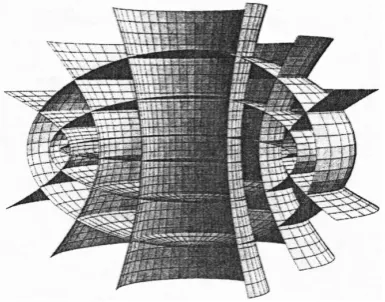
[image:2.595.277.470.556.707.2]Enderlein [3] has depicted this coordinate net as shown in Figure 1.
DOI: 10.4236/jmp.2019.105036 517 Journal of Modern Physics A slice of the ellipsoid of revolution should make understandable the position of the coordinate lines and is shown in Figure 2.
[image:3.595.235.513.114.343.2]Figure 2. The elliptic-parabolic coordinate system.
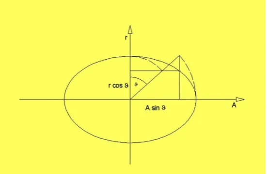
In order to work out the meaning of the quantities in (2.2), we first deal in detail with the ellipses by reducing the problem to two dimensions
1' 2'
cos sin
x r
x A
ϑ ϑ =
= (2.7) Evidently r and A are the minor and major axes of the confocal ellipses. Al-though the coordinate r is not the radial direction of the system, the historical notation is maintained. The meaning of the quasi-polar angle ϑ can be found in Figure 3.
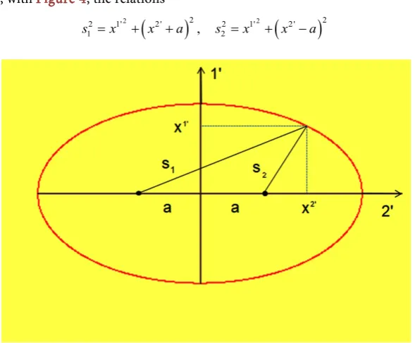
[image:3.595.237.513.520.699.2]DOI: 10.4236/jmp.2019.105036 518 Journal of Modern Physics Further properties of the ellipses can be made accessible. If one draws the foc-al rays s1 and s2 from the foci of an ellipse to any point of the ellipse, one
finds, with Figure 4, the relations
(
)
(
)
2 2 2 2
2 1' 2' 2 1' 2'
1 , 2
s =x + x +a s =x + x −a
[image:4.595.227.522.111.354.2]Figure 4. Focal rays and eccentricity.
and then
1 2
2 2 2 2 2 2
1 2
sin , sin
sin cos
s A a s A a
s s A a r a
ϑ ϑ
ϑ ϑ
= + = −
= − = +
Thus, the fundamental quantities of the ellipses can be represented as the geometric and the arithmetic means of the focal rays
1 2 1 2, s s2
s s A +
Λ = = (2.8) The factor ahead of dr2 in (2.4) has to be examined in more detail. At ϑ=0,
i.e. at the minor axes of the ellipses, this factor
(
r2+a2cos2ϑ
) (
r2+a2)
is equal to 1, so that the radial part of the metric isreduced to dr2. At ϑ =π 2 the factor is r A2 2 . It follows that the radial arc
element has the value dA at this position. Thus, the quantity Λ A describes the varying distance of two neighboring confocal ellipses; at the minor axis this dis-tance is dr and at the major axis it is dA. This proves that several quantities of the geometry show this behavior, so that it is sufficient to compute these quantities at one of the minor axes, and then to multiply them by this factor, which we call
elliptical factor. However, these quantities offer a further surprise. With
2 2
2 2 2 2
2 1 2sin 1 , 2
R a a
a
A A
ϑ
ω σ
ω
AΛ
= = − = − = (2.9)
al-DOI: 10.4236/jmp.2019.105036 519 Journal of Modern Physics ready makes available the fundamental quantities for a rotating system. Not sur-prisingly, the Kerr geometry is built on an elliptical system.
From the equations of the ellipses and hyperbolae one gets the nonvanishing components of the curvature vectors
{
,0,0 ,}
{
0, ,0 ,}
3, 2 3 sin cosE H
E H E rA H a
α α
ρ
ρ
ρ
ρ
ρ
ρ
ϑ
ϑ
Λ Λ
= = = = − (2.10)
1, 2,3
α= is a tetrad index. The two vectors are perpendicular and are in each case tangent to the other family of curves. In this way the term radial is defined in this geometry. “Radial” refers to the directions which are specified by the tan-gents of the hyperbolae.
Facing the 3rd dimension, σ =Asinϑ is the curvature radius of the circles, the parallels of the ellipsoid of revolution. Finally, one has the curvatures of the coordinate lines
1 ,0,0 , 0, 1 ,0 , 0,0,1
E H
Bα ρ Nα ρ Cα σ
= = =
(2.11)
These quantities and their derivatives constitute the curvature equations of the system and satisfy the “field equations” Rαβ =0 , where Rαβ is the
3-dimensional Ricci for the parabolic-hyperbolic system.
3. The Kerr Surface
So far, we have associated geometrical meaning to the quantities of the flat me-tric (2.4), written in elliptic-hyperbolic coordinates. Now we return to the meme-tric (2.2), but we omit the timelike part. To explain the factor αS =Aδ in the radial arc element, we extend (2.5) with the extra dimension x0'
0' 1' 2' 3' tan d cos sin cos sin sin x r x r x A x A ε ϑ ϑ ϕ ϑ ϕ = − = = =
∫
(3.1)We will show that (3.1) provides an embedding of a surface into a 5-dimensional flat space, which we will discuss in more detail.
We define the angle ε by
2 2
sin r M, cos , tan Mr
A r A
δ
ε ε ε
δ
= − = = − , (3.2)
where ε has the orientation cw. Evidently tanε tends to infinity for δ =0. The solution to r of this equation is
2 2
H
r =M + M −a (3.3)
H
r settling the event horizon of the Kerr model. Finally, the integral in (3.1) reads as 0' 2 2 2 d 2 H r r Mr x r
r a Mr
=
+ −
DOI: 10.4236/jmp.2019.105036 520 Journal of Modern Physics The solution does not have a closed form; however, the integral can be eva-luated numerically. If one suppresses the φ-dimension the surface appears as shown in Figure 5.
[image:6.595.248.501.130.330.2]Figure 5. The surface with suppressed φ-dimension.
The surface looks like a “funnel”. Its horizontals are ellipses. The ellipse fixed by rH is the ellipse at the waist of the funnel and is the “end” of the geometry.
0
δ = marks the limit of the model. The projection of the funnel onto the base
planes shows ellipses crossed by hyperbolae. Thus, the integral lines (3.4) have a 1st and 2nd curvature. We note that the ansatz (3.1) still does not provide the Kerr metric. We have to add further ingredients to gain the metric (2.2). But Figure 5
shows a lot of the properties that the genuine Kerr surface will have.
This surface is closely related to the Schwarzschild surface, i.e. Flamm’s para-boloid. For a=0 the metric (2.2) is reduced to the Schwarzschild metric and the elliptical coordinate system breaks down to the spherical polar system. The integral lines are parabolae and their projections onto the base plane are straight lines.
If one extends to the φ-dimension and suppresses the ϑ-dimension, the sur-face builds up on concentric circles and is even more closely related to Flamm’s paraboloid.
We must bear in mind that dr is the increase of the minor axes of the el-lipses on the base plane. In contrast,
1
dx =a rRd (3.5) is the distance of two neighboring ellipses and depends on the angle ϑ. If one pulls up elliptical cylinders on two of such ellipses, one can see that their cutting curves with the surface do not lie on the horizontal slices of the surface. During a circulation on the surface the points of the cutting curve oscillate. From
( )
0' 1 1
DOI: 10.4236/jmp.2019.105036 521 Journal of Modern Physics one gets the augment of the height of the surface into the extra dimension.
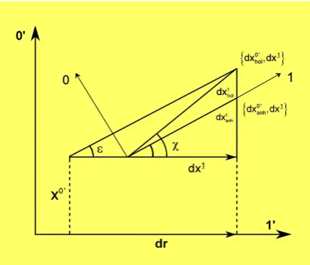
It is evident that the tangent related to the auxiliary angle χ which points to the next higher point of the surface depends on the angle ϑ. A short calculation would show that one does not arrive at the desired seed metric by using (3.6) ei-ther. For our model only the horizontal elliptical slices of the surface are of im-portance. If one follows the normal vector of the surface along an ellipse, one will discover that this vector also oscillates on its way, because the walls of the surface are round about differently scarped. In order to be able to use the surface, it has to be equipped with an additional structure. On the minor axes of the el-lipses the elliptical factor is aR =1 and the geometry is Schwarzschild-like. That is where we start: we define a rigging vector in such a way that it coincides with the normal vector at this position, and that it always encloses the same an-gle with the base plane during its circulation. Then this rigging vector is no longer vertical to the surface and its vertical planes are no longer tangent to the surface. The family of all of these planes—and if one adds the φ-dimension, the family of the 3-dimensional hyperplanes—represents our graphic space, if we assume that we live in such a world. Those hyperplanes are anholonomic, as will be shown.
Now we replace the holonomic differential (3.6) by an anholonomic one
( )
0 ' 1
dxanh= −tanεa rR , dϑ r= −tan dε x (3.7) that is no longer integrable. We call the family of hyperplanes that are orthogon-al to these differentiorthogon-als and that are no longer V3-forming physical surface. It is the area of all possible physical observations.
However, the structure of the [r, φ]-part of the surface is simple. On this patch no elliptical properties and hence no anholonomies arise. It corresponds to Flamm’s paraboloid of the Schwarzschild geometry. Sharp [7] has searched for such a surface for ϑ =π 2. However, he did not start from the seed metric, but incorporated rotational parts of the Kerr metric into his computations. Hence, his result differs substantially from ours. From
2 2 2 2
2 0' 1' 2' 3'
ds =dx +dx +dx +dx
one indeed obtains with
(
)
22 2 2 2 2 2 2 2
2
ds tan 1 dr d A sin d
A
ε
Λϑ
ϑ ϕ
= + + Λ +
the desired seed metric, which serves as a basis for the actual Kerr metric. From the definition aS =δ A in (2.3) and the introduction of cosε δ= A, and with the definition of the elliptical factor aR we obtain the spatial part of the Kerr metric
2 2 2 2 2 2 2
ds =αS Ra rd + Λ dϑ +A sin ϑ ϕd (3.8) and the surface related to this metric we will call Kerr surface.
The anholonomic construction will be examined in more detail. Figure 6
DOI: 10.4236/jmp.2019.105036 522 Journal of Modern Physics two “radial” vectors, the vector1 d 1
hol
x in the tangent planes of the surface and the associated vector d 1
anh
[image:8.595.261.485.130.321.2]x in the anholonomic hyperplanes, which have the same projections onto the basic plane.
Figure 6. Holonomic and anholonomic differentials.
Having explained the structure of the Kerr metric, we return to Equation (3.2) and recognize that the ascent of the integral curve is −tanε = ∞ for δ =0, i.e. at ε =π 2. Thus, the integral lines are normal to the base plane at rH. For
0
ε= the ascent is tanε =0 and the geometry will be flat in the infinite. We also read from (3.2) that for vanishing eccentricity a of the ellipses, i.e.
0
a= , we get with A r=
2 2 1 1
sin , cos 1 ,
cos 1 2
M M
r r M
r
ε ε
ε
= − = − =
−
Thus, in this case sinε is the velocity of a freely falling observer in the Schwarzschild model and 1 cosε the related Lorentz factor.
We have good reasons to interpret
2
2 1
sin ,
1
S S
S
r M A
v
A r v
ε α
δ
= = − = =
− (3.9) as velocity of a freely falling observer in the exterior field of a rotating stellar ob-ject and αS as the correlated Lorentz factor of this motion. r A is the ratio of the axes of the ellipses. This means that the velocity of a freely falling observer depends on position in relation to the ellipses.
At the waist of the Kerr surface
(
δ =0)
is vR= −1, i.e. the observer has (asymptotically) reached the velocity of light, measured with his proper time in-dependently of his former position on the ellipse. Since we do not assume that1All the other components of the vector except the mentioned one vanish in the local reference
DOI: 10.4236/jmp.2019.105036 523 Journal of Modern Physics velocities higher than the velocity of light can occur, we have to realize that the waist of the Kerr surface is not only a geometrical limit, but also a physical limit of the model. No object can cross the event horizon rH.
In addition, we have to bear in mind that a radial motion in the fields of ro-tating objects in free fall is not possible. Since frame dragging acts on observers, the motion of an observer will get a circular component. Due to Einstein’s law of composition of velocities the velocity of an observer will asymptotically reach the velocity of light before reaching the event horizon. The limit in this case is the ergosphere, as we have shown in [5] [6]. Our point of view is supported by similar circumstances in the Schwarzschild model. In contrast to the claims of Misner, Thorne, and Wheeler [8], we have shown in several papers and in [5] [6]
that an observer starting from an arbitrary position can reach the Schwarzschild radius only asymptotically in infinite proper time. We have also shown [9] that the surface of a collapsing star, described by the Schwarzschild interior solution, collapses eternally, reaching the inner horizon of the model asymptotically in in-finite proper time. Thus the final state of a collapsing non-rotating stellar object is an ECO (Eternally Collapsing Object) [10].
Thus, if we believe that this geometrical description of a rotating star is a good description of Nature, we have to dismiss the possibility of the formation of ro-tating black holes. We have supplemented the Kerr solution with an interior so-lution [11] [12], which has the property of developing into the interior Schwarz-schild solution for a=0. However, we have made no attempt to implement a collapse for this model and we have not found any effort in the literature in this regard. If such an approach is possible, a RECO (Rotating Eternally Collapsing Object) would be expected.
4. Curvatures of the Elliptic-Hyperbolic Geometry
So far we have shown that the Kerr model is based on an elliptic-hyperbolic sys-tem, endowed with an integral surface with elliptical horizontals, which could be envisaged as an elliptically deformed Flamm’s paraboloid. The Boyer-Lindquist coordinate system, with its curved coordinate lines, contributes to Einstein’s field equations, which have little to do with the physical content of the model but are incorporated in the connexion coefficients of the physical quantities and must be treated for this reason.
Still suppressing the timelike part of the seed metric, we have to deal with the curvature vectors
{
}
{
}
{
}
{
}
,0,0,0 , 0, ,0,0 ,
0,0, ,0 , 0,0,0, , 0,1,2,3
S E
a S a E
H C
a H a C a
ρ ρ ρ ρ
ρ ρ ρ ρ
= =
= = = (4.1)
E
ρ and ρH are the components of the curvature vectors of the ellipses and hyperbolae. They have been mentioned in (2.10). ρC = =σ Asinϑ is the radius of the circles of the parallels of the ellipsoids of revolution. ρS is the curvature radius of the integral lines and was calculated in [5] [6]2.
DOI: 10.4236/jmp.2019.105036 524 Journal of Modern Physics The inverse quantities of (4.1) are the curvatures in vector form. Their tetrad components related to BL-coordinates are
{
}
{
}
{
}
{
}
1 1 1
1,0,0,0 , sin ,cos ,0,0 , 0,0,1,0 ,
1 sin sin ,cos sin ,cos ,0 ,
a a a
S E H
a
C
M B N
C
ε
ε
ρ
ρ
ρ
ε
θ
ε
θ
θ
ρ
= = =
= (4.2)
where
sinθ = r sin , cosϑ θ = Acosϑ
Λ Λ . (4.3)
All the quantities in (4.2) obey the structure
2
d 1 1 0 dr r r+ = .
The “field equations” for B, N and C refer to the elliptic-hyperbolic system and drop out from Einstein’s field equations. But we cannot omit these quanti-ties, because we need them for the covariant derivative of the physical quantities which we will discuss later on.
We start with the detailed discussion of these quantities. The quantity B is re-lated to the curvature radii ρE of the ellipses. We know that the curvature B is normal to the ellipses. Thus, we introduce an auxiliary reference system
" 0",1", 2"
a = and suppress the φ-dimension for the sake of simplifying the problem. In this system B has only one component
{
}
" 0,1,0 1
a
E
B = ρ , (4.4)
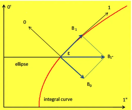
as seen in Figure 7. For the sake of simplicity, the holonomic Kerr surface is used for some of the quantities for the drawings.
[image:10.595.243.506.483.701.2]DOI: 10.4236/jmp.2019.105036 525 Journal of Modern Physics It is evident that B1" can be split into two components with respect to the BL
system. One component (B1) is tangent to the integral curve and the other one
(B0) is normal to the curve, pointing in the 0-direction, i.e. the local
extradi-mension. Thus, one has
{
sin ,cos ,0}
1a
E
B ε ε
ρ
= . (4.5)
1 1 cos
E
B ε
ρ
= is the very component an observer can measure in his physical space, B0 is hidden to him.
Furthermore, we ask for the components of B in the Cartesian coordinate sys-tem of the embedding space. We obtain
{
}
' 0,cos ,sin 1
a
E
B θ θ
ρ
= . (4.6)
The components of Ba' are depicted in Figure 8:
[image:11.595.241.517.290.585.2]Figure 8. Horizontal splitting of B1".
From the figure it can be seen that θE is the angle of ascent of the curvature ra-dius of the ellipse and can be calculated by (4.3), setting θE =θ. With
{
ρ θE, E}
one can describe the elliptical system instead of
{ }
r,ϑ . Alternatively, one can describe the hyperbolic system with{
ρ θH, H}
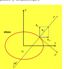
, where θH =π 2−θE, bearing in mind that the ellipses and hyperbolae are orthogonal trajectories.DOI: 10.4236/jmp.2019.105036 526 Journal of Modern Physics Again, the auxiliary reference system is chosen in such a way that the 1’’-direction is tangent to the hyperbolae and the 2’’-direction is tangent to the ellipses. Thus, the curvature N has only one component in this system
{
}
'' 0,0,1 1
a
H
N = ρ (4.7)
as can be seen in Figure 9.
[image:12.595.238.510.180.419.2]Figure 9. Horizontal splitting of N.
In the Cartesian reference system N has the components
{
}
{
}
' 0, sin ,cos 1 0,cos , sin 1
a H H
H H
N θ θ θ θ
ρ ρ
= − = − −
, (4.8) recalling that ρH is a negative quantity and that θH =π 2−θ . In the BL sys-tem one has
{
0,0,1}
1a
H N
ρ
= . (4.9)
Next, we discuss the quantity C, which is related to the curvature radii of the circular parallels of the ellipsoids of revolution, i.e. ρC = =σ Asinϑ. Thus, C has only one component in the Cartesian system lying in the 2'-direction
{
}
' 0,0,1 1
a
C = σ . (4.10)
But two components occur in the auxiliary system a"
{
}
'' 0,sin ,cos 1
a
C θ θ
σ
= (4.11)
DOI: 10.4236/jmp.2019.105036 527 Journal of Modern Physics Figure 10. Horizontal splitting of C.
Finally, the component C1" has a projection onto the tangent of the integral
curve and onto the local extradimension
{
sin sin ,cos sin ,cos}
1a
C ε θ ε θ θ
σ
= . (4.12)
This is depicted in Figure 11.
[image:13.595.238.510.471.699.2]DOI: 10.4236/jmp.2019.105036 528 Journal of Modern Physics Recall that the angle ε is cw and thus C0 is pointing into the opposite
direc-tion of the local extradimension x0.
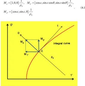
The quantity M still needs to be discussed. It does not belong to the ellip-tic-hyperbolic system, but to the integral surface. M is related to the curvature radii of the integral lines and has the components
{
}
{
}
{
}
'
''
1 1
1,0,0 , cos ,sin cos ,sin sin ,
1 cos ,sin ,0
a a
S S
a
S
M M
M
ε
ε
θ
ε
θ
ρ
ρ
ε
ε
ρ
= =
= . (4.13)
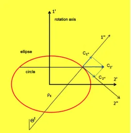
[image:14.595.242.529.154.446.2]Figure 12. Vertical splitting of M.
M is situated in the direction of the local extradimension as shown in Figure 12. The quantity is only important for the use of 5-dimensional covariant derivatives. Since we do not use this formalism in this paper, we will not discuss this quanti-ty in detail.
So far we have intuitively derived various representations of the fundamental quantities by drawing figures. For the interested reader we note the transforma-tion matrices
''
'' '
'
cos sin 1
sin cos , cos sin
1 sin cos
cos sin cos sin sin sin cos cos cos sin
sin cos
a a
a a
a a
ε ε
ε ε θ θ
θ θ
ε ε θ ε θ
ε ε θ ε θ
θ θ
Λ = − Λ =
−
Λ = −
−
(4.14)
DOI: 10.4236/jmp.2019.105036 529 Journal of Modern Physics
2 2 2 2 2 2 2 2 2 2 2 2
ds =αS Ra rd + Λ dϑ +A sin ϑ ϕd +aSρSdiψ . (4.15) Therein dx4 is evidently defined by
4
dx =i td =ρSdiψ . (4.16) The metric is written in the original Hilbert notation with index 4, i.e. (++++) and the timelike element is interpreted as an arc on a pseudo circle, shown as a pseudoreal representation in Figure 13.
[image:15.595.243.505.187.386.2]Figure 13. The geometrical definition of time.
We have to bear in mind that when using a real and an imaginary axis the pseudo circle cannot be drawn or even imagined. The time we measure with our clocks is the real accessory number of an imaginary angle and the flow of time is the arc of a pseudo circle. The infinite past and the infinite future are the points on the 45˚ axes in the figure.
Sometimes another pseudoreal representation is used, a hyperbola instead of a circle. This has the advantage that the infinite can be better visualized, but the hyperbola shows a position-dependent curvature, while the pseudo circle has a constant curvature, including the infinite. Therefore a pseudo circle is also called
hyperbola of constant curvature. Unfortunately the pseudoreal representation with hyperbolae misleads some authors to take the hyperbolae literally, but this hinders a geometric explanation of the Kerr metric with the help of an embed-ding.
We call the factor aS in (4.15) gravitational factor. Its derivative leads us to the force of gravity 1 1 tan
S
E ε
ρ
= and is a member of the Ricci-rotation coefficients of the seed model. From (2.3) we see that if the rotational parameter is a=0 the elliptical factor is aR =1, and also A r= . Thus, taking ρS from (2.3) we
Schwarz-DOI: 10.4236/jmp.2019.105036 530 Journal of Modern Physics schild geometry. In this case, 1 1 tan
S
E ε
ρ
= will be the gravitational force of the Schwarzschild model. Since the angle ε is cw, the gravitational force is pointing inwards.
Now we analyze the geometrical meaning of this quantity. In the 5-dimensional embedding space it has the components
{
}
{
}
'
1 1, tan ,0 cos , sin ,0 1 , cos 1
1,0,0
cos
a
S S S
a
S E
E
ε ε ε
ρ ρ ρ ε
ρ ε
= − = − −
= −
(4.17)
From Figure 14
[image:16.595.219.531.148.490.2]Figure 14. The gravitational force.
we can see that ρScosε are the projections of the curvature radii ρS into the extradimension 0' of the embedding space. E0' is the inverse of ρScosε. It is split into the components with respect to the local BL reference system a. E1
is tangent to the integral curves. It is the very quantity a physical observer can experience. The second component is hidden to him.
Having explained the fundamental quantities of the seed metric with curva-tures, we reformulate the metric with the help of curvature radii. For the flat el-liptic-hyperbolic system we have
2 2 2 2 2 2 2
ds =ρ θHd H +ρ θEd E +ρ ϕCd and for the seed metric with ρψ =ρScosε we have
2 2 2 2 2 2 2 2 2
DOI: 10.4236/jmp.2019.105036 531 Journal of Modern Physics
5. The Field Equations
All the quantities B N C E, , , discussed in the previous section are members of the Ricci-rotation coefficients and satisfy the subequations of Einstein’s field eq-uations. For a detailed discussion we again refer to [5] [6]. Here we restrict our-selves to noting some relations. For the elliptic-hyperbolic basic system we ob-tain
2 2
1|1 1 1 , 2|2 2 2
B +B B = Ω N +N N = −Ω .
The occurrence of the quantity Ω is the second surprise of the ellip-tic-hyperbolic system. It is a second-rank tensor describing rotational effects which we will meet with the genuine Kerr metric. Evidently the sum of the above equations vanishes. In a covariant form the curvature equations of the ellip-tic-hyperbolic system can be written as
2 2 3
|| || 0, || 0, 1,2,3,4.
s s s s s s
s s s s s s
N N N B B B C C C s
+ + + = + = =
(5.1)
Thus, these subequations of the Ricci drop out from Einstein’s field equations. The only quantity of physical interest is the force of gravity. It is contained in Einstein’s field equations with the structure
4
||
s s
s s
E −E E , (5.2)
i.e. the field of gravity is coupled to itself, due to the non-linearity of Einstein’s field equations.
To get the Equations (5.1) and (5.2) we have skipped the tedious procedure of
dimensional reduction, i.e. getting rid of all 0-components and all 0-derivatives of the fundamental quantities, and we have restricted ourselves to the flat basic system, the shadow on the horizontals of the Kerr surface. Thus, we are left with 4-dimensional quantities and their graded derivatives [5] [6]. We will only briefly remark on how the quantity Ω comes into the theory. We have
exten-sively used coordinate systems with ellipses and their curvature vectors, which represent a kind of polar system. But we have to bear in mind that the pole of this system is not fixed, but moves on the evolute of the ellipses, if the curvature vector moves on the ellipses. Thus, the change of ρE and of the related curva-ture B has two contributions, the one by motion of the tip of the curvature vec-tor on the evolvente, the other one by motion of the tail of the curvature vecvec-tor on the evolute. The latter produces the term Ω2. The same holds for
H ρ and the related curvature N.
The seed metric does not provide a vacuum solution, it is an auxiliary metric, a forerunner to better explain the Kerr metric. Thus, we will not continue with this model but will turn to study the rotational effects in the next section.
6. Rotation
DOI: 10.4236/jmp.2019.105036 532 Journal of Modern Physics
3' 3' 4' 2 4'
3 4 3 4
3 3 4 2 4
3' 4' 3' 4'
2
, , ,
, , ,
, sin
R R R R
R R R R
i i
i i
a a
A A
α α ω α ωσ α
α α ω α ωσ α
ω ωσ ϑ
Λ = Λ = Λ = − Λ =
Λ = Λ = − Λ = Λ =
= =
. (6.1)
Operating on the coordinate indices of the tetrads, we get the genuine Kerr metric
2 2 2 2
2 1 2 3 4 2 3 4
4
d d d d d d d
d d d
R R S R R
S
s x x x i x a i x x
x i i t
α α ωσ α ωσ α
ρ ψ
= + + + + − +
= = (6.2)
ω is the angular velocity and ωσ the orbital velocity of an observer subjected to frame dragging by the field of a rotating source. The 4-bein system obtained in this way is named system C after Carter and is one of the preferred reference systems attributed to the Kerr model. The coordinate system is oblique-angled, the Carter tetrads are mutually perpendicular by definition.
In contrast, if we perform a Lorentz transformation
3' 3' 4' 4'
3 R, 4 R , 3 R , 4 R
L =α L =iα ωσ L = −iα ωσ L =α (6.3) operating on the tetrad indices of the seed metric, we obtain instead of
2 2
2 2 2 2 2 2 3 2 4 3
ds =αS Ra rd + Λ dϑ +dx +a xSd , dx =Asin dϑ ϕ (6.4) the metric
2 2
2 2 2 2 2 2 3 4 3 4
ds =αS Ra rd + Λ dϑ +αRdx +iα ωσR dx + − iα ωσR dx +αR Sa xd (6.5) which differs from the genuine Kerr metric (6.2) only by the position of the gra-vitational factor aS concerning the last brackets. Although the two metrics are very similar, they have a quite different physical interpretation. While in (6.2) the rotation is inherent, the metric (6.5) is still static, but observers are rotating around the source producing the exterior field. We use the similarities of the metrics to make clearer the structure of the rotational effects of the Kerr metric.
It will be shown that the metrics (6.2) and (6.5) exhibit the same fundamental rotational structures. Since it turns out that (6.5) is much easier to treat, we make use of this property, and we will compare the results for both metrics at the end of the section.
Evidently, it is sufficient to consider the [3,4]-piece of the metric. We make a further simplification: we put aS =1αS =1, i.e. we switch off the gravitational force. Thus, we are left only with rotational effects and we get
2 2
2 2 2 2 2 3 4 3 4
DOI: 10.4236/jmp.2019.105036 533 Journal of Modern Physics has a differential rotation law, a property of the model being a condition for a physically functional rotating model.
From the Lorentz factor αR from the orbital motion we get with
|
1 R R
F D
α α α
α
α = + (6.7) the relations
2 2 2 2
|
,
R R
Fα =α ω σσα Dα =α ωω σα . (6.8)
Evidently the first quantity in the above formulae is the relativistic generaliza-tion of the centrifugal force; it is normal to the rotageneraliza-tion axis. The second emerges from the differential law of rotation ω ω=
( )
r . It has only one compo-nent and is pointing inwards. From the orbital velocity we derive{
}
2 2
[ ] |
2 R , R , 0,0,1
Hαβ = iα ωσα βc Dαβ =iα ω σα cβ cβ = . (6.9)
H is antisymmetric and is the relativistic generalization of the Coriolis field strength. The quantity D is a consequence of the differential law of rotation and is asymmetric (D3β =0). Both quantities are summarized to
H D
βα αβ αβ
Ω = − − . (6.10) By the decomposition of Ω into an antisymmetric and a symmetric part
[ ] ( )
H D D
βα αβ αβ αβ
Ω = − + − (6.11)
one obtains the total rotational field strength and the deformation field strength.
Ω is the very quantity we met at the end of Section 5 when considering the mo-tions of the curvature vectors on the evolutes of the ellipses and hyperbolae. The symmetric part represents the shears
{
}
( || ) ( ), m 0,0,0,1
uα β = −Dαβ u = (6.12) that should be understood as the observers sliding past each other on account of the different speeds on neighboring circular paths, whereby shears of the sur-rounding volume elements arise. The new quantities satisfy the relations
|| n , || , 1,2,3, 1,2,3,4
m n m
u u =F uα β = Ωαβ α = m= , (6.13) where the double strokes indicate the ordinary covariant derivative in tetrad re-presentation.
From Einstein’s field equations Rmn ≡0 one obtains equations of Maxwell type
4
4
||
[ ] ||
0
2 0
m m mn
m m nm
mn nm
m m
F F F
F
− − Ω Ω =
Ω + Ω = (6.14)
The centrifugal force is coupled to the field energy, which is composed of qu-adratic terms. The quantity Ω is coupled to the Poynting vector 2 [ ]nm
m F
Ω .
DOI: 10.4236/jmp.2019.105036 534 Journal of Modern Physics
4 4 4
4
[ || ] [ || ] [ || ] 3[ ]3
[ || ] [ ]
0, 2 0
0
m n m n m n m n
mn s mn s
F D F
F
+ = + Ω Ω =
Ω + Ω = (6.15)
are satisfied. They are Maxwell-like as well. The conservation laws
(
)
(
)
4
[ ] ||
0, 2 0
m mn nm
m nm m n
F F F
t
∂ + Ω Ω = Ω =
∂ (6.16)
are valid. In the formulae above we used the 4th graded derivative [5] [6]. It cor-responds to the spatial covariant derivative.
If we drop the restriction aS =1 we obtain the gravitational force Em en-tering Einstein’s field equations with the structure (5.2). In the above equations
E will accompany the centrifugal force Fm, which has the opposite orientation but not the same direction.
Now we compare the simplified equations with the one of the genuine Kerr metric
|| || 0
s s rs C
s s C sr
E +F − Ω Ω = (6.17)
4 4 4 4
[ || ]m n [ || ]m n 0, [ || ]m n 2 3[n n]3, [ || ]m n 0
F +D = F = Ω Ω E = (6.18)
4
[ || ] [ ] [ ] 0
C C C
mn s mnDs mn sE
Ω = Ω − Ω = (6.19)
4
[ ] ||
|4 0, 2 0,
s C sr C ms C C
C s C rs C s m n n n
E E E E E F
+ Ω Ω = Ω = = +
(6.20)
The tag C indicates the quantities of the Carter system, where some of the new quantities differ from the quantities of the simplified system by a factor. In the first brackets one finds terms quadratic in the field strengths. They represent the field energy and are conserved. The second brackets contain the divergence-free Poynting vector. We recognize that the simplified rotational piece of the Kerr model is very close to the genuine Kerr theory.
For a better understanding of the above equations we make a further simplifi-cation by putting ω=const.. In this case the quantities Dα and Dαβ,
refer-ring to the differential rotation law, vanish. Only the centrifugal force Fα and
the vorticity Hαβ remain. The field equations for these quantities are
Max-well-like.
First, we define the axial vector
, 2
i
Hα αβγH Hαβ i αβγH
βγ γ
ε ε
= − = (6.21)
and we obtain
{
}
2 , cos ,sin ,0
R
Hα=α ωτα τα = θ θ . (6.22)
Having transformed this vector into Cartesian coordinates we have
{
}
' 2 ', ' 1,0,0
R
Hα =α ωτα τα = . 6.23)
Since τα' is a unit vector lying in the 1’-direction, it is parallel to the rotation
DOI: 10.4236/jmp.2019.105036 535 Journal of Modern Physics
Figure 15. The axial unit vector.
Thus, one can write in vector notation
2 2 2, 0
0, 2
div rot
div rot
= + =
= = ×
F F H F
H H F H (6.24)
wherein div is the 3-dimensional covariant divergence and rot the 3-dimensional covariant rotator. The centrifugal force F has as a source the field energy, the Coriolis force H is coupled to the Poynting vector. The conservation laws take the form
(
2 2 2)
0, div(
2)
0t
∂ + = × =
∂ F H F H . (6.25)
Evidently, the field equations have a similar structure to the Maxwell equa-tions of electrodynamics. The genuine Kerr Equaequa-tions (6.14)-(6.20) also have almost the same structure. The similarity of gravitation and electrodynamics was first discovered by Lense and Thirring [13] and Thirring [14] [15] [16] in weak field approximation and treated in general form by Hund [17]. In the last decades this problem was investigated by many authors and called gravi-to-electromagnetism (GEM).
7. Kerr Interior Solution
Several authors have tried to complement the Kerr solution with an interior model. Although the results have been unsatisfactory to date, the search for a solution is still ongoing. We [11] [12] have proposed an interior solution which goes over into the Schwarzschild solution by setting the rotational parameter a
to zero. For this model we did not solve Einstein’s field equations but instead constructed the model in terms of geometrical methods.
DOI: 10.4236/jmp.2019.105036 536 Journal of Modern Physics
2 2 2 2
2 1 2 3 4 2 3 4
1 2 3
4 2 2 2
d d d d d d d
d d , d d , d d ,
1
d d , , 1
R R T R R
I R
R R
R
s x x x i x a i x x
x a r x x
x i t a
a
α α ωσ α ωσ α
α ϑ σ ϕ
α ω σ
= + + + + − +
= = Λ =
= = = −
(7.1)
has the same form as the exterior (2.2). It differs by the geometrical factor
2 2
2
1 , 1
I I
I
r a
a
α = = −
R (7.2)
and the gravitational factor
(
2)
22 2 2 2
2
2 2 2 2
1 1 2 cos cos 2
, cos 1 , cos 1
T g g g
g g
g g I
g a
r a r r a
r a
η
η
η
η
−
= + Φ − Φ
+
Φ = = − = − =
− R R
(7.3)
R and the rotational parameter a are constants. All quantities with the
sub-script g are the constant values of the variables at the boundary surface matching the exterior solution. Evidently, for a=0, 2 1
g
Φ = the gravitational factor has the form of the Schwarzschild interior solution. The spacelike piece of this mod-el is a cap of a sphere with radius R and the aperture angle ηg. The cap matches Flamm’s paraboloid at rg =Rsinηg.
The embedding for the spacelike piece of the Kerr model is
0' 2 2
1' 2' 3' cos sin cos sin sin x r x r x A x A ϑ ϑ ϕ ϑ ϕ = ± − = = = R (7.4)
depicted in Figure 16.
[image:22.595.238.510.410.705.2]DOI: 10.4236/jmp.2019.105036 537 Journal of Modern Physics From this surface a band has to be cut off and the remaining surface has to be matched horizontally to the auxiliary surface of the Kerr metric. R is the
ra-dius of the circular arc at the minor axes of the ellipses. All individual ‘radial’ curves have hyperbolic contributions in their properties. For r=0,A a= the horizontal ellipses reduce to a distance which is clamped by the common foci of the ellipses. If one now adds the third dimension, these points rotate through ϕ. For ϑ =π 2 a circle emerges. The radius of curvature of the ellipses is zero on this circle and the assigned field strengths are infinitely large. This is the Kerr ring singularity.
[image:23.595.248.499.309.505.2]Since the junction condition is satisfied, both solutions, the interior and the exterior, match, as can be seen in Figure 17. The Kerr interior shows centrifugal, Coriolis, and gravitational forces, which can be geometrically explained as we have done with the forces of the exterior solution. The interior has a complicated stress-energy-momentum tensor, consisting of gravitational energy, current, and stresses. All that is treated in [5] [6] in detail.
Figure 17. The complete Kerr solution.
8. Summary
We have revisited the Kerr model with the methods of tetrads. These are ortho-gonal local reference systems. The components of the field quantities represented in these systems are measurable quantities and have a clear geome-trical or physical meaning. We have visualized the curvature of space with sur-faces and have demonstrated how these quantities emanate from geometrical structures with several drawings.
DOI: 10.4236/jmp.2019.105036 538 Journal of Modern Physics
Conflicts of Interest
The author declares no conflicts of interest regarding the publication of this paper.
References
[1] Kerr, R. P. (1963) Phys. Rev. Lett. 11, 237-238. https://doi.org/10.1103/PhysRevLett.11.237
[2] Boyer, R. H., Lindquist, R. W. (1965) Proc. Camb. Phil. Soc. 61, 531 [3] Enderlein, J. (1997) Am. J. Phys. 65, 897-902.
https://doi.org/10.1016/0003-4916(78)90079-9 [4] Krasinski A. (1978) Ann. Phys.112, 22-40.
https://doi.org/ 10.1016/0003-4916(78)90079-9 [5] Burghardt, R. (2005) Spacetime Curvature.
http://members.wavenet.at/arg/EMono.htm
[6] Burghardt, R. (2005) Raumkrümmung. http://members.wavenet.at/arg/Mono.htm [7] Sharp, N. A. (1981) Can. J. Phys. 59, 688-692. https://doi.org/10.1139/p81-086 [8] Misner, C. W., Thorne K. S., Wheeler J. A., (1973) Gravitation, San Francisco. [9] Burghardt, R. (2015) Journ. Mod. Phys. 6, 1895-1907.
https://doi.org/10.4236/jmp.2015.613195
[10] Mitra, A., (2006) Black Holes or Eternally Collapsing Objects: A Revue of 90 Years of Misconception. Focus of Black Hole Research. Nova Science Publishers, New York, 1-97.
[11] Burghardt, R. (2007) Sitz. Ber. Leib. Soz. Wiss. 92, 51-60. http://members.wavenet.at/arg/WKerr7.pdf
[12] Burghardt, R. (2007) Sitz. Ber. Leib. Soz. Wiss. 92, 61-70,
http://members.wavenet.at/arg/WKerr8.pdf
[13] Lense, J., Thirring H. (1918) Phys. Z. 19, 156-163. [14] Thirring, H. (1918) Phys. Z. 19, 33-39.