Predicting the effects of human developments on individual dolphins to understand potential long term population consequences

1

Predicting the effects of human developments on individual dolphins to

understand potential long-term population consequences

Enrico Pirotta*a, John Harwoodb,c, Paul M. Thompsond, Leslie Newe, Barbara Cheneyd, Monica Arsob, Philip S. Hammondb, Carl Donovanc, David Lusseaua

a

Institute of Biological and Environmental Sciences, University of Aberdeen, Aberdeen AB24 2TZ, UK

b

Scottish Oceans Institute, East Sands, University of St Andrews, St Andrews KY16 8LB, UK c

Centre for Research into Ecological and Environmental Modelling, University of St Andrews, St Andrews KY16 9LZ, UK

d

Lighthouse Field Station, Institute of Biological and Environmental Sciences, University of Aberdeen, Cromarty IV11 8YL, UK

e

Washington State University, 14204 Salmon Creek Avenue, Vancouver WA, 98686, USA

*

Corresponding author: Enrico Pirotta, Institute of Biological and Environmental Sciences, University of Aberdeen, Tillydrone Avenue, Aberdeen AB24 2TZ, UK. Email: [email protected]. Phone: +353 (0)83 8491393

2

Abstract

Human activities that impact wildlife do not necessarily remove individuals from populations. They may also change individual behaviour in ways that have sub-lethal effects. This has driven interest in developing analytical tools that predict the population consequences of short-term behavioural responses. In this study, we incorporate empirical information on the ecology of a population of bottlenose dolphins into an individual-based model that predicts how individuals’ behavioural dynamics arise from their underlying motivational states, as well as their interaction with boat traffic and dredging activities. We simulate the potential effects of proposed coastal developments on this population and predict that the operational phase may affect animals’ motivational states. For such results to be relevant for management, the effects on individuals’ vital rates also need to be quantified. We investigate whether the relationship between an individual’s exposure and the survival of its calves can be directly estimated using a Bayesian multi-stage model for calf survival. The results suggest that any effect on calf survival is likely small and that a significant relationship could only be detected in large, closely-studied populations. Our work can be used to guide management decisions, accelerate the consenting process for coastal and offshore developments and design targeted monitoring.

Keywords

3

1. Introduction

Management decisions regarding the effects of human activities on wildlife should ideally be taken before targeted populations start declining. However, it is hard to predict the long-term consequences of anthropogenic impacts [1], especially for long-lived marine predators [2]. As a result, it might be too late to act effectively by the time a negative trend in population size is detected [3].

There are modelling tools to assess the viability of populations following the direct removal of individuals [4]. However, human activities do not necessarily kill or injure exposed animals. They may, instead, sub-lethally disturb their activity patterns (e.g. [5–7]). Recent research has focused on how changes in behaviour alter the dynamics of populations, with the aim of developing a framework to predict the population consequences of disturbance before conservation status is compromised [8,9]. This requires a mechanistic understanding of the relationship between changes in an animal’s activity and its vital rates, such as survival probability and reproductive success [10–12]. This relationship can be disrupted if disturbed individuals are unable to maintain their energy balance and lose condition [8,13]. Behaviourally-mediated cascades that lead to long-term effects on population dynamics have been documented in response to changes in predation risk (e.g. [14]). There is a growing body of evidence showing that animals perceive human disturbance as a form of predation risk [15,16], implying that responses to disturbance may invoke similar cascades.

Any behavioural response to disturbance will depend on an individual’s internal state, its perceived risks and habitat quality [17,18]. Previous work has shown that behavioural temporal dynamics can be modelled successfully through the integration of an individual’s motivational states, which combine the effects of external stimuli and physiological needs [19–21]. Since motivations are unobservable, mechanistic models are required, and agent- or individual-based models have been used for this purpose [22,23]. Predicted changes in an animal’s internal states can then be linked to its energy balance and condition to understand how its allocation of energy to survival or reproduction will be impacted [8,10]. However, information on individual condition is rarely available for wild animals. Previous work has attempted to link changes in behaviour directly to fitness [11,12], but the success of this approach depends on the sample size available to inform the models as well as on the severity of the disturbance effects [24]. Detecting such relationship may prove difficult if individual heterogeneity is large and the effect size is small, but the precise sampling requirements for a robust assessment are unclear.

4 interval: 162-253) bottlenose dolphins Tursiops truncatus (hereafter ‘dolphins’ or ‘bottlenose dolphins’) that range along the East coast of Scotland has been the subject of long-term research [26,27], and information is available on their distribution and habitat preferences [28,29], as well as the reproductive history of individual animals [30]. Dolphins distribute close to the coast, with marked individual differences in habitat use [28], and appear to forage in discrete patches in their habitat associated with specific bathymetric and tidal features [29]. Some individuals consistently use areas within the inner Moray Firth [31], which has been designated as a Special Area of Conservation (SAC) for the species under the European Habitats Directive (92/43/EEC). Marine industrial developments have been proposed in this area, because of its strategic importance for traditional and renewable energy exploitation in the North Sea. These will involve increased boat traffic and coastal development (e.g. construction or enlargement of harbours, with associated piling, dredging and dumping activities), which could compromise the population’s “favourable conservation status” (a regulatory target that the UK must maintain under European legislation). Such uncertainty can lengthen the time it takes to reach a consenting decision for these developments. These uncertainties can be reduced using modelling approaches that provide robust and easy to communicate predictions of possible long-term effects. Previous work has developed a theoretical framework to model the consequences of human disturbance on individual animals [22], but such tools need to have a strong empirical grounding in order to provide robust management advice.

The aim of this study is to construct a predictive tool for assessing the risks to the conservation status of a dolphin population posed by new developments. First, we develop an individual-based model for bottlenose dolphin behavioural dynamics in the Moray Firth, based on the interplay of internal motivational states. We use that model to estimate individual dolphins’ exposure and motivational states during a six-year baseline period, and then predict future changes in exposure and motivational states resulting from proposed industrial developments. Finally, we test whether there is any association between the estimated exposure of individual females to disturbance and the survival of their calves (Fig. 1).

2. Material and Methods

2.1 Individual-based model

5 to spend energy) that resulted from the integration of internal and external stimuli and that regulated its behavioural decisions [19,20]. Dolphin movements across their range were then determined on the principles of habitat selection and foraging theory. When the motivation to acquire energy was higher than the motivation to spend energy, we assumed that animals would try to meet their energy needs by preferentially selecting locations where they could find suitable foraging opportunities [34]. When their motivation to spend energy was higher, we used the observed pattern of habitat use in a given year to determine an individual’s movements, on the assumption that the observed home range was the result of its attempts to meet its needs other than foraging (e.g. travelling, mating and other social interactions, resting or minimizing perceived risks). We assumed that dolphins perceived anthropogenic disturbance as a form of predation risk [15]. Therefore, any behavioural response would emerge indirectly from disturbance affecting the individuals' motivation to spend energy. While building on the concepts developed in [22] and [23], our model shifts the focus to the habitat preferences and autonomous decision-making regarding movement and activity of individual animals. In addition, we replace the tuned parameters used in [22] with ecological parameters estimated from empirical data. The model is described using the updated ODD (Overview, Design concepts, Details) protocol [35,36]. The sections “Design concepts”, “Initialisation” and “Submodels” are provided in the Supplementary material, where model assumptions are also discussed. The code for constructing the individual-based model is included in the Supplementary material.

2.1.1 Purpose

The purpose of our individual-based model was to simulate individual dolphins' behavioural dynamics, track their motivational states across time, and assess the effect of exposure to boat traffic and construction activity on individuals' activity budget and motivations.

2.1.2 State variables and scales

6 traffic (mean daily number of hours spent by boats in each cell), and presence or absence of dredging activities.

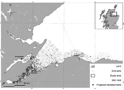
We simulated between 27 and 35 individual dolphins, depending on the year (Table S.1 in Supplementary material). While individuals in this population range along the entire East coast of Scotland [26], we simulated only those that were known to spend most of their time in the inner Moray Firth area [31,37], and for whom an estimate of home range was available [28]. They included 17 known females. We used a grid of 959, 1 km by 1 km cells enclosing suitable dolphin habitat in the Moray Firth [28] (Fig. 2). For each simulation, the model was run 500 times for 612 discrete six-hour time steps, resulting in a time horizon of 153 days. Six six-hours was the mean duration of an activity bout, as indicated by the patterns of autocorrelation in the residuals of previous models of dolphin foraging in the area [29,32] (Fig. S.1 in Supplementary information). The 153 days covered the period between the 1 May and 30 September each year, corresponding to the mark-recapture sampling period for this population.

2.1.3 Process overview and scheduling

7 environmental covariates in the following day. For each simulation, we recorded each individual’s overall mean motivational states, its mean motivation states in the last week of the simulation (i.e. its final state), the number of times its motivations were completely satisfied or dissatisfied, the number of boat interactions and the mean activity budget. Details of the submodels and model equations are provided in the Supplementary material.

2.1.4 Input data

External inputs to the model included estimates of each individual's home range for the given year, the estimated spatio-temporal distribution of dolphin foraging activity, the predicted distribution of boat traffic across the study area under baseline and disturbed conditions, the estimated effect of boat presence and number on animals' motivations, and the estimated effect of dredging activities.

We modelled six baseline conditions, corresponding to the summers between 2006 and 2011. We used the estimated individual home ranges for each summer from [28], the dynamic distribution of foraging activity predicted as a function of environmental conditions from [29], and the number of boat hours predicted for each cell on each day by the boat model described in [22,28]. The distribution of foraging activity was used as a measure of the daily suitability of each cell for dolphin foraging, and was calculated using the model from [29] and the values of the environmental covariates on each day. The spatio-temporal distribution of boat traffic was assumed to be the same across different years (Fig. 2). [32] provided estimates of the effect of boat presence and numbers on foraging activity. We compared the number of boat interactions between years and individuals using a Poisson Generalized Linear Model (GLM). The motivational states did not follow a Gaussian distribution. Therefore, we transformed the response by adding 1.0001, and used a Gamma GLM to analyse the variability of the motivational states between years and individuals. This transformation was required because the Gamma distribution is bounded at 0 (not included), while motivations had a lower bound of -1. We also simulated a series of disturbance conditions. In particular, we considered the construction and operational phase of three proposed coastal development sites in the area (port of Ardersier, Invergordon, Nigg Bay; Fig. 2). The details of these developments are provided in Environmental Statements that are available on the website of the Scottish Government (http://www.scotland.gov.uk/Resource/0041/00416136.pdf,

http://www.scotland.gov.uk/Resource/0042/00423292.pdf,

http://www.scotland.gov.uk/Resource/0043/00438787.pdf). A summary of the key activities

8 taking place. The developments also involved disposal of dredged material at sea and some piling activities, but these could not be included in the model because of the absence of data on the animals' potential responses. The effects of construction and operation of the three sites were modelled using the environmental conditions and individual home ranges observed in 2009 and 2010, since previous work showed that these years reliably exemplified different dolphin ranging patterns among the six years analyzed [28].

2.1.5 Simulated population scenarios

We simulated three scenarios of population status to calibrate the individual-based model parameters. These scenarios were based on the mean individual motivational states at the end of the simulated summer season under mean home range and foraging conditions and with a baseline condition of boat traffic (see Supplementary material):

Scenario 1) All individuals were completely satisfied with their motivational states (i.e. their motivational states were close to -1);

Scenario 2) Individuals were on average satisfied with their motivational states (i.e. the mean value of the motivations was -0.5);

Scenario 3) On average, individuals were not satisfied nor dissatisfied with their motivational states (i.e. the mean value of the motivations was 0, and the population was therefore on the verge of a possible decline caused by its individuals not being able to meet their needs).

2.2 A multi-stage model for calf survival

We tested whether the exposure to boat traffic and the motivational states of individual females estimated by the individual-based model had an effect on their ability to successfully raise their calves, i.e. if they affected calf survival probability. We used model predictions in the six baseline years in association with information from long-term photo-identification studies carried out in the Moray Firth SAC [38] and in the southern part of the population's range [37]. On average, 28 (Moray Firth SAC) and 12 dedicated surveys (southern part of the range) were conducted each summer (May-September) in the study period (2006-2011). The studies record the occurrence of each identified dolphin in the study area and whether or not they were accompanied by calves. We focused on the sighting history of calves that were consistently associated with the same female [39], because we anticipated that disturbance was more likely to affect calf survival rather than female pregnancy rate [40,41].

9

 Stage 1: newborn (age 0, born in that same year);

 Stage 2: age 1 or 2 years;

 Stage 3: age 3 or more;

 Stage 4: dead.

We grouped calves of age 1 and 2 together in order to reduce the number of parameters in the model, and because we expected calves to be at least partially dependent on maternal milk until at least age 3 [42]. Because calves could be lost once the association with their mother loosened (due to the limited amount of marking on their fins), we decided to introduce an observation model under which the calf's stage could be misclassified. In particular, a calf that was classified as dead could, in reality, be in stage 2 or 3 but unrecognised. We considered the sighting histories of 20 calves that were associated with 14 females included in our individual-based model (i.e. females for which we had information on exposure to disturbance) during 2006 – 2012 (Table S.2 in Supplementary material). We tested for an effect of the predicted exposure to boat interactions across the summer, the mean and final motivation to acquire energy, and the number of maternal satisfactions and dissatisfactions with the motivation to acquire energy experienced by the females on the transition of the dependent calf to the subsequent stage. We fitted the hierarchical model in a Bayesian framework. Additional analytical details and assumptions are provided in the Supplementary material.

Given the small sample size available to inform the multi-stage model, we designed a simulation study to assess the bias on the estimates of the transition probabilities and the effect size required to retain the effect of boat exposure. Further details on the simulation study are provided in the Supplementary material.

3. Results

3.1 Individual-based model

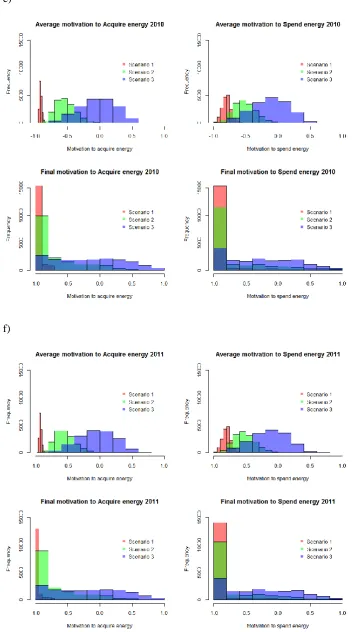
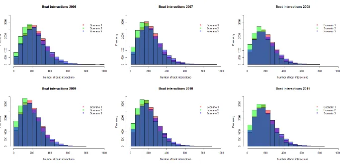
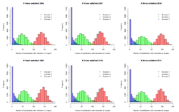
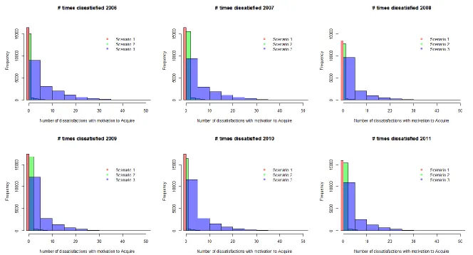
The estimated mean and final motivational states for the years 2006-2011, as well as the number of satisfactions and dissatisfactions, confirmed the expected differences between the three population status scenarios resulting from the adjustment of the cost-benefit parameters (Fig. S.2-S.5). Differences between years were much smaller, although the Poisson GLM showed that the number of boat interactions changed significantly (χ2= 310727; df=5; p<2.2×10-16). The model also highlighted significant differences between individuals (χ2= 111376; df=34; p<2.2×10-16). The motivations were found to vary consistently among years (e.g. mean motivation to acquire energy: χ2= 5654; df=5;

p<2.2×10-16) and among individuals (e.g. mean motivation to acquire energy: χ2= 1600; df=34;

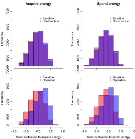
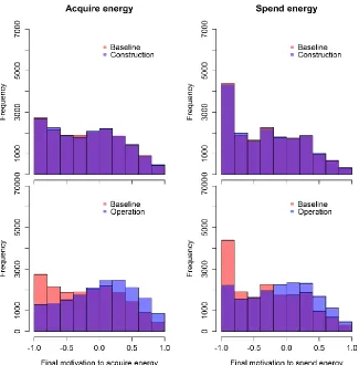
10 The model did not predict any substantial change in either the overall exposure of the animals or their motivational states as a result of the increase in boat traffic and dredging activity during the construction phase of the three development sites (Fig. 3, S.6 and S.7). However, during the operational phase, a relatively small increase in the number of boat interactions experienced by each individual across the summer (median difference = 9 (scenario 1) – 16 (scenario 3)) was sufficient to cause a shift of the motivational states towards dissatisfaction (Fig. 3, S.6 and S.8). This increase was more evident under scenario 3, in which the population was on the verge of a possible decline caused by its individuals not being able to meet their needs (mean difference in mean motivation to acquire energy = 0.19), than under scenario 1, in which individuals were completely satisfied (mean difference = 0.003). In particular, the mean across the 500 simulations became greater than zero, suggesting overall dissatisfaction for both motivational states. We did not detect any relevant difference between the predicted scenarios run using 2009 versus 2010 ranging patterns in either the construction or operational phases.

3.2 Calf multi-stage model

The MCMC chains quickly converged and there appeared to be no issues with autocorrelation. The effects of the number of boat interactions on the transition probabilities between stages were found to be negligible, based on the mean values of the corresponding indicator variables (wβ1 < 0.5; wβ2 < 0.5). The result did not change when effects on the mean and final motivation to acquire energy were tested. Therefore, we concluded that there was no detectable association between the mothers' predicted exposure and motivational states and the survival of their calves. We removed these effects from the model and re-ran the MCMC. The resulting matrix of posterior transition probabilities was:

P =

showing a high probability of surviving to age 1 (p12). The matrix of posterior misclassification probabilities for the observation model was:

11

4. Discussion

Effective management of human developments in the marine environment requires an approach that protects marine mammal populations while allowing for the sustainable use of marine resources. Human activities do not necessarily lead to the direct injury or death of the exposed individuals, but sub-lethal changes in individual behaviour can result in changes in individual vital rates, mediated by the alteration of the animals’ energy balance and condition [8,10–12]. Similar behaviourally-mediated cascading effects have been observed in response to variation in the spatio-temporal patterns of predation risk, which can cause substantial changes in an entire community [14]. It is therefore important to develop analytical frameworks that allow such effects to be predicted before the population declines, in order to inform effective regulation of anthropogenic disturbances [8]. Here, we describe a model framework, constructed using a robust evidence base, that can be used to address these issues and facilitate management decisions.

We developed an individual-based model for bottlenose dolphin behavioural ecology that combines previous individual- and population-level empirical observations to inform the animals’ unobservable motivational states. Our work builds on similar approaches developed for this and other dolphin populations [22,23], but, crucially, our focus is on individuals rather than schools. We used information on the ranging pattern of a selection of well-known individual animals to estimate their spatially-explicit exposure to disturbance and to make predictions of their state. The heterogeneity in home ranges and, consequently, exposure was assumed to be representative of the portion of the population consistently using the study area, and thus provide an estimate of the range of potential effects on the individuals, even when the mean effect is overall negligible. Understanding the variability around the absence of an effect is critical if any long-term population trend is to be predicted, because the contribution of different individuals to the demography of the population might be unbalanced [43,44].

12 satisfy their motivational states. At the moment, we have no means to assess where the mean motivation in the population lies on this continuum, and therefore we cannot make predictions of the population’s ability to compensate for these potential changes.

In the absence of data on the current mean motivational state of the population, we simulated three possible underlying scenarios. Therefore, our results represent a gradient of increasing precaution that takes account of known uncertainties and whose predictions are relatively easy to communicate to decision-makers. However, in order to ensure the favourable conservation status of the population, estimates of motivational states need to be translated into measures of individuals' demographic contributions [8]. Developing a bioenergetic model to predict changes in individual condition would require an unreasonable number of assumptions, as few data are available on the diet and energetic strategies of this population, or on prey availability and distribution. Rather than introducing additional uncertainty, we decided to ignore intermediate changes in condition and directly investigate the link between disturbance and calf survival. We used a Bayesian multi-stage model to assess whether the exposure and motivational states of the mothers could have a detectable effect on the transition of their calves between critical growth stages. We were unable to detect any significant effect, which is not surprising given the small sample size compared to the expected individual differences in reproductive output [42,44]. In addition, the overall stability of the population size [27] implies that any current detrimental effect on calf survival is likely small.

13 The trajectory of this bottlenose dolphin population is currently stable [26,27] and, despite the biases deriving from the small sample size, the simulation study suggested that the proposed developments are unlikely to cause a substantial disruption of calf survival (or, at least, the effect cannot be distinguished from natural individual heterogeneity). In light of these results, the condition of individuals should now be monitored, so that any deterioration following increased exposure to disturbance can be rapidly detected, before it translates into longer-term changes in the population's trend. The growth rate of immature animals and the accumulation of energy stores in the blubber could represent good proxies of individual condition, but new techniques to measure them at sea are required. We are currently investigating photogrammetric methods to estimate calf growth [45,46]. Research is also ongoing to identify a suitable technique to estimate blubber stores from photographic data, as has been done for pinnipeds [47]. In addition, accelerometry data collected by electronic tags have been used to estimate pinnipeds’ body condition and its variation at sea [48,49]. While accelerometer sensors have been successfully combined with suction-cap tags for free-ranging cetaceans [50], future research should aim at improving attachment techniques to allow for longer-term sampling than is currently possible and for more effective remote transmission of the data. Capture and release of wild animals for direct measurements is possible at a small number of sites, where some of these indirect techniques could be validated [46].

14 unsampled or less known species, where tolerance towards disturbance could also vary. For example, it could be assumed that species with comparable life histories will adopt the same strategies in response to a disturbance source or a changing habitat, and will make similar decisions to allocate their energy. Marine mammal reproductive strategy is often placed along a continuum ranging from capital breeding, in which individuals rely on stored reserves during the reproductive period, to income breeding, in which individuals have to forage during lactation [54]. Our framework was developed for an income breeding species, but the idea of underlying motivations driving the engagement in observable activities can also be applied to a capital breeder on its feeding ground [55].

Conclusion

Approaches that link short-term physiological and behavioural responses to disturbance to long-term population consequences could provide an overarching framework for investigating wildlife populations’ viability in a changing environment [8,9,56]. We show how information on the behavioural ecology of a population can be integrated into an individual-based model that predicts an individual’s behavioural dynamics and any potential change in its vital rates resulting from disturbance. This model could easily be adapted to other small populations of marine mammals where similar information has been collected. While some mechanistic links still need to be appropriately informed, our work can be used to guide management decisions, accelerate the consenting process for coastal and offshore developments, and identify knowledge gaps that need to be filled using appropriate monitoring methods.

Acknowledgements

This work received funding from the MASTS pooling initiative (the Marine Alliance for Science and Technology for Scotland). Detailed acknowledgements are provided in the Supplementary material.

References

1. Maxwell, D. & Jennings, S. 2005 Power of monitoring programmes to detect decline and recovery of rare and vulnerable fish. Journal of Applied Ecology42, 25–37.

15 3. Turvey, S. T. et al. 2007 First human-caused extinction of a cetacean species? Biology Letters

3, 537–540. (doi:10.1098/rsbl.2007.0292)

4. Wade, P. R. 1998 Calculating limits allowable human-caused mortality of cetaceans and pinnipeds. Marine Mammal Science14, 1–37. (doi:10.1111/j.1748-7692.1998.tb00688.x) 5. Duchesne, M., Côté, S. D. & Barrette, C. 2000 Responses of woodland caribou to winter

ecotourism in the Charlevoix Biosphere Reserve, Canada. Biological Conservation 96, 311– 317. (doi:10.1016/S0006-3207(00)00082-3)

6. Kerley, L. L., Goodrich, J. M., Miquelle, D. G., Smirnov, E. N., Quigley, H. B. & Hornocker, M. G. 2002 Effects of roads and human disturbance on Amur tigers. Conservation Biology16, 97–108. (doi:10.1046/j.1523-1739.2002.99290.x)

7. Pirotta, E., Brookes, K., Grahamh, I. M. & Thompson, P. M. 2014 Variation in harbour porpoise activity in response to seismic survey noise. Biology Letters 10, 20131090. (doi:10.1098/rsbl.2013.1090)

8. New, L. F. et al. 2014 Using short-term measures of behaviour to estimate long-term fitness of southern elephant seals. Marine Ecology Progress Series 496, 99–108. (doi:10.3354/meps10547)

9. National Research Council 2005 Marine mammal populations and ocean noise: determining

when noise causes biologically significant effects. US National Academy of Sciences,

Washington, DC.

10. Béchet, A., Giroux, J.-F. & Gauthier, G. 2004 The effects of disturbance on behaviour, habitat use and energy of spring staging snow geese. Journal of Applied Ecology 41, 689–700. (doi:10.1111/j.0021-8901.2004.00928.x)

11. McClung, M. R., Seddon, P. J., Massaro, M. & Setiawan, A. N. 2004 Nature-based tourism impacts on yellow-eyed penguins Megadyptes antipodes: does unregulated visitor access affect fledging weight and juvenile survival? Biological Conservation 119, 279–285. (doi:10.1016/j.biocon.2003.11.012)

12. Kight, C. R. & Swaddle, J. P. 2007 Associations of anthropogenic activity and disturbance with fitness metrics of eastern bluebirds (Sialia sialis). Biological Conservation138, 189–197. (doi:10.1016/j.biocon.2007.04.014)

13. Schick, R. S., Kraus, S. D., Rolland, R. M., Knowlton, A. R., Hamilton, P. K., Pettis, H. M., Kenney, R. D. & Clark, J. S. 2013 Using hierarchical Bayes to understand movement, health, and survival in the endangered north Atlantic right whale. PloS one 8, e64166. (doi:10.1371/journal.pone.0064166)

14. Fortin, D., Beyer, H. & Boyce, M. 2005 Wolves influence elk movements: behavior shapes a trophic cascade in Yellowstone National Park. Ecology86, 1320–1330.

15. Frid, A. & Dill, L. 2002 Human-caused disturbance stimuli as a form of predation risk.

Conservation Ecology6, 11.

16. Beale, C. M. & Monaghan, P. 2004 Human disturbance: people as predation-free predators?

16 17. Bejder, L., Samuels, A., Whitehead, H., Finn, H. & Allen, S. 2009 Impact assessment research: use and misuse of habituation, sensitisation and tolerance in describing wildlife responses to anthropogenic stimuli. Marine Ecology Progress Series 395, 177–185. (doi:10.3354/meps07979)

18. Gill, J. A., Norris, K. & Sutherland, W. J. 2001 Why behavioural responses may not reflect the population consequences of human disturbance. Biological Conservation 97, 265–268. (doi:10.1016/S0006-3207(00)00002-1)

19. McFarland, D. J. & Sibly, R. M. 1975 The behavioural final common path. Philosophical

Transactions of the Royal Society of London Series B: Biological Sciences270, 265–93.

20. Zucchini, W., Raubenheimer, D. & MacDonald, I. L. 2008 Modeling time series of animal behavior by means of a latent-state model with feedback. Biometrics 64, 807–815. (doi:10.1111/j.1541-0420.2007.00939.x)

21. Schliehe-Diecks, S., Kappeler, P. M. & Langrock, R. 2012 On the application of mixed hidden Markov models to multiple behavioural time series. Interface Focus 2, 180–189. (doi:10.1098/rsfs.2011.0077)

22. New, L. F. et al. 2013 Modeling the biological significance of behavioral change in coastal bottlenose dolphins in response to disturbance. Functional Ecology 27, 314–322. (doi:10.1111/1365-2435.12052)

23. Pirotta, E., New, L., Harwood, J. & Lusseau, D. 2014 Activities, motivations and disturbance: An agent-based model of bottlenose dolphin behavioral dynamics and interactions with tourism in Doubtful Sound, New Zealand. Ecological Modelling 282, 44–58. (doi:10.1016/j.ecolmodel.2014.03.009)

24. Osenberg, C., Schmitt, R., Holbrook, S. J., Abu-Saba, K. E. & Flegal, A. R. 1994 Detection of environmental impacts: natural variability, effect size, and power analysis. Ecological

Applications4, 16–30.

25. Nowacek, D. P., Thorne, L. H., Johnston, D. W. & Tyack, P. L. 2007 Responses of cetaceans to anthropogenic noise. Mammal Review37, 81–115.

26. Cheney, B. et al. 2013 Integrating multiple data sources to assess the distribution and abundance of bottlenose dolphins Tursiops truncatus in Scottish waters. Mammal Review43, 71–88. (doi:10.1111/j.1365-2907.2011.00208.x)

27. Cheney, B. et al. 2014 Long-term trends in the use of a protected area by small cetaceans in relation to changes in population status. Global Ecology and Conservation 2, 118–128. (doi:10.1016/j.gecco.2014.08.010)

28. Pirotta, E., Thompson, P. M., Cheney, B., Donovan, C. R. & Lusseau, D. 2015 Estimating spatial, temporal and individual variability in dolphin cumulative exposure to boat traffic using spatially explicit capture-recapture methods. Animal Conservation 18, 20–31. (doi:10.1111/acv.12132)

17 30. Arso, M. 2015 Population ecology of bottlenose dolphins (Tursiops truncatus) off the East

coast of Scotland. PhD dissertation, University of St Andrews.

31. Wilson, B., Reid, R. J., Grellier, K., Thompson, P. M. & Hammond, P. S. 2004 Considering the temporal when managing the spatial: a population range expansion impacts protected areas-based management for bottlenose dolphins. Animal Conservation7, 331–338.

32. Pirotta, E., Merchant, N. D., Thompson, P. M., Barton, T. R. & Lusseau, D. 2015 Quantifying the effect of boat disturbance on bottlenose dolphin foraging activity. Biological Conservation

181, 82–89.

33. Pirotta, E., Laesser, B. E., Hardaker, A., Riddoch, N., Marcoux, M. & Lusseau, D. 2013 Dredging displaces bottlenose dolphins from an urbanised foraging patch. Marine Pollution

Bulletin74, 396–402. (doi:10.1016/j.marpolbul.2013.06.020)

34. Redfern, J. V. et al. 2006 Techniques for cetacean-habitat modeling. Marine Ecology Progress

Series310, 271–295. (doi:10.3354/meps310271)

35. Grimm, V. et al. 2006 A standard protocol for describing individual-based and agent-based models. Ecological Modelling198, 115–126. (doi:10.1016/j.ecolmodel.2006.04.023)

36. Grimm, V., Berger, U., DeAngelis, D. L., Polhill, J. G., Giske, J. & Railsback, S. F. 2010 The ODD protocol: A review and first update. Ecological Modelling 221, 2760–2768. (doi:10.1016/j.ecolmodel.2010.08.019)

37. Quick, A. N., Arso, M., Cheney, B., Islas, V., Janik, V., Thompson, P. M. & Hammond, P. S. 2014 The east coast of Scotland bottlenose dolphin population: Improving understanding of ecology outside the Moray Firth SAC. UK Department of Energy and Climate Change Report 14D/086.

38. Cheney, B., Graham, I. M., Barton, T. R., Hammond, P. S. & Thompson, P. M. 2014 Site Condition Monitoring of bottlenose dolphins within the Moray Firth Special Area of Conservation: 2011-2013. Scottish Natural Heritage Commissioned Report No. 797.

39. Grellier, K., Hammond, P., Wilson, B., Sanders-Reed, C. A. & Thompson, P. M. 2003 Use of photo-identification data to quantify mother calf association patterns in bottlenose dolphins.

Canadian Journal of Zoology81, 1421–1427. (doi:10.1139/Z03-132)

40. Currey, R. J. C., Dawson, S. & Slooten, E. 2009 Survival rates for a declining population of bottlenose dolphins in Doubtful Sound, New Zealand: an information theoretic approach to assessing the role of human. Aquatic Conservation: Marine and Freshwater Ecosystems 19, 658–670. (doi:10.1002/aqc)

41. Bejder, L. 2005 Linking short and long-term effects of nature-based tourism on cetaceans. PhD dissertation, Dalhousie University, Canada.

42. Mann, J., Connor, R., Barre, L. & Heithaus, M. 2000 Female reproductive success in bottlenose dolphins (Tursiops sp.): life history, habitat, provisioning, and group-size effects.

Behavioral Ecology11, 210–219.

18 time. Proceedings of the Royal Society of London. Series B: Biological Sciences273, 547–555. (doi:10.1098/rspb.2005.3357)

44. Henderson, S. D., Dawson, S. M., Currey, R. J. C., Lusseau, D. & Schneider, K. 2014 Reproduction, birth seasonality, and calf survival of bottlenose dolphins in Doubtful Sound, New Zealand. Marine Mammal Science30, 1067–1080. (doi:10.1111/mms.12109)

45. Fearnbach, H., Durban, J., Ellifrit, D. & Balcomb, K. 2011 Size and long-term growth trends of Endangered fish-eating killer whales. Endangered Species Research 13, 173–180. (doi:10.3354/esr00330)

46. Hart, L., Wells, R. & Schwacke, L. 2013 Reference ranges for body condition in wild bottlenose dolphins Tursiops truncatus. Aquatic Biology18, 63–68. (doi:10.3354/ab00491) 47. Waite, J., Schrader, W., Mellish, J. & Horning, M. 2007 Three-dimensional photogrammetry

as a tool for estimating morphometrics and body mass of Steller sea lions (Eumetopias

jubatus). Canadian Journal of Fisheries and Aquatic Sciences64, 296–303.

(doi:10.1139/F07-014)

48. Schick, R. S. et al. 2013 Estimating resource acquisition and at-sea body condition of a marine predator. Journal of Animal Ecology82, 1300–1315. (doi:10.1111/1365-2656.12102)

49. Biuw, M. et al. 2007 Variations in behavior and condition of a Southern Ocean top predator in relation to in situ oceanographic conditions. Proceedings of the National Academy of Sciences

of the United States of America104, 13705–10. (doi:10.1073/pnas.0701121104)

50. Johnson, M. P. & Tyack, P. L. 2003 A digital acoustic recording tag for measuring the response of wild marine mammals to sound. IEEE Journal of Oceanic Engineering28, 3–12. 51. Crain, C. M., Kroeker, K. & Halpern, B. S. 2008 Interactive and cumulative effects of multiple

human stressors in marine systems. Ecology Letters 11, 1304–15. (doi:10.1111/j.1461-0248.2008.01253.x)

52. Wells, R. S. et al. 2004 Bottlenose dolphins as marine ecosystem sentinels: developing a health monitoring system. EcoHealth1, 246–254.

53. Wells, R. S. 1991 The role of long-term study in understanding the social structure of a bottlenose dolphin community. In Dolphin societies: discoveries and puzzles (eds K. Pryor & K. Norris), pp. 199–225. Berkeley: University of California Press.

54. Stephens, P., Boyd, I., McNamara, J. & Houston, A. 2009 Capital breeding and income breeding: their meaning, measurement, and worth. Ecology90, 2057–2067.

55. Christiansen, F. & Lusseau, D. In press. Linking behaviour to vital rates to measure the effects of non-lethal disturbance on wildlife. Conservation Letters.

56. Cooke, S. J. et al. 2014 Physiology, behavior, and conservation. Physiological and

19

Figures

22

Supplementary material

1. Additional details of the individual-based model

Design concepts

Basic principles: Dolphin movements across their range were based on the principles of habitat selection and foraging theory, i.e. we assumed that animals would try to maximize their energy intake by preferentially selecting locations where they could find suitable foraging opportunities [1]. When the animals were not driven by the motivation to acquire energy, we used the observed pattern of habitat use in a given year to determine an individual’s movements, on the assumption that this was the result of its attempts to meet its overall needs (e.g. mating and other social interactions, resting or minimizing perceived risks). Dolphin behavioural dynamics were modelled under the assumption that each individual animal had a set of motivational states that resulted from an integration of internal and external stimuli, and which regulated its behavioural decisions [2,3]. Finally, the interactions between boats and dolphins were modelled on the assumption that anthropogenic disturbance was perceived as a form of predation risk [4].

Emergence: An individual's desired activity emerged from its motivational states. The choice of its next location was then determined by its desired activity and by the individual's home range.

Adaptation: Individuals' activities changed in response to the variation of their underlying motivational states.

Objectives: The motivations were an individual's measure of its condition. Each animal aimed at keeping the levels of the two motivational states below zero, which indicated satisfaction with its state and the possibility to maintain a balanced energy budget.

Learning: There was no explicit learning process underlying dolphins' behaviour, but the continuous update of the motivational states represented a way to integrate an individual's previous experience. Prediction: Dolphins perceived boats as a potential risk and were therefore assumed to be affected by their presence and numbers. When dolphins were driven by the motivation to acquire energy, their movements were assumed to result from our predictions of the foraging opportunities they would find across their range.

23

Interaction: There was no interaction among individual dolphins directly implemented in the simulations.

Stochasticity: The choice of an individual's location at each time step arose stochastically from the properties of the individual’s home range and the foraging surface. This process simulated environmental complexity as well as other unaccounted factors (e.g. social dynamics) that could affect an individual's decision-making. The number of boats in a given location in a given interval was determined as a random draw based on the number of daily boat hours in that cell and the maximum number of boats occurring concurrently.

Collectives: There were no collectives in the model.

Observation: For each simulation, we recorded dolphins' overall mean motivational states, the mean motivation state in the last week of the simulation (its final state), the number of times each individual was completely satisfied or dissatisfied with its motivations, the number of boat interactions and the mean activity budget.

Initialization

Dolphins' initial motivational states were randomly drawn from a uniform distribution U(-0.1,0.1). The initial date was always 1 May.

Submodels

The motivational states of each individual dolphin were unit-less measurements varying between -1 (indicating complete satisfaction with that motivation) and 1 (indicating complete dissatisfaction). We considered two competing motivations: the motivation to spend energy (i.e. to perform any activity that involves energy expenditure) and the motivation to acquire energy (i.e. to forage, since this is the only activity that warrants energy intake). At the beginning of each time step t, the larger of the two motivations determined the desired activity (either to spend or to acquire energy) in that time step. Spending energy was possible in every cell of the grid, and therefore a dolphin whose motivation was to spend energy only had to select a new location xi,t based on its home range:

xi,t ~ Multinom (1,ri),

24

If the desired activity was acquiring energy, we constructed a new probability surface. [6] provided an estimate of the probability of foraging across the study area in year y and day d (fy,d), given that the animals were there. Therefore, the probability that an individual was in a given location and could forage (fri,y,d) was calculated as:

fri,y,d = ri × fy,d.

fri,y,d did not sum to 1, as foraging opportunities were not necessarily always available. The individual’s location in that time step was then drawn as:

xi,t ~ Multinom (1, fri,y,d).

If no foraging location was available (i.e. no foraging grid cell was drawn), the actual activity was again spending energy, and the individual’s location was drawn from its home range. Otherwise, the animal would move to xi,t where it could acquire energy. In this case, the six-hour bout was split into 120 three-minute intervals, and the number of boats present in cell x in each interval v (bt,v,x) was calculated as:

bt,v,x ~ B(max, pd,x),

where max was the maximum number of boats observed at any time in each location and was assumed to be 13 based on visual observations in the area [7]. pd,x was the probability of a boat passing in location x on day d in one three-minute interval and was calculated as:

pd,x = hd,x / 4 × 60 / pass / 120 / max,

where hd,x was the predicted number of hours during which boats would be present in cell x on day d, and was extracted from the boat model described in [8,9]; this was divided by 4 to obtain the predicted number of boat-hours per six-hour time step, and multiplied by 60 to transform it into minutes. pass was the median duration of a boat passage in each location obtained from the work described in [7], and 120 was the number of intervals per bout. This probability guaranteed that the mean expected number of boat hours per cell per day coincided with the predictions of the original boat model.

25

was indeed a reflection of the true effect on the motivations, while the variability around this relationship represented context-dependent plasticity. Otherwise, the animals would not be able to maintain their energy balance in the long-term, and we would observe a declining trend in the population. Boat presence is expected to act as an external stimulus in opposition to an individual’s internal energetic needs, so it was assumed to increase the motivation to spend energy. We therefore took the estimated reduction in foraging probability as a function of the number of boats [7] and assumed that the opposite relationship could be used to inform such effect on the motivation to spend energy. The motivation to spend energy ms,t for individual i was then updated as:

ms,t,i = ms,t,i + effectb,

where effectb was the predicted change in motivation when the number of boats was b. The two motivational states were then compared again, and if the motivation to spend energy had surpassed the motivation to acquire energy, the individual would spend energy in that three-minute interval. Otherwise, it would keep acquiring energy.

At the end of each six-hour bout, the vector of motivational states mt,iwas updated based on the actual activity of individual i across the bout t:

mt,i = mt-1,i + 120 × Aat,

where at was a vector of length two indicating the activity budget for bout t; the first element of the vector was the proportion of intervals where the individual was acquiring energy, while the second was the proportion of intervals where the individual was spending energy. 120 was the number of three-minute intervals in each bout, and A was a two by two matrix with the cost-benefits of the activities on the motivational states in each three-minute interval. When the motivational states exceeded -1 or 1, their value was re-adjusted within these constraints.

Spending energy was assumed to reduce the corresponding motivation and increase the motivation to acquire energy. Vice versa, acquiring energy was assumed to decrease the corresponding motivation and increase the motivation to spend energy. The size of the cost-benefits in A was adjusted via model calibration. We simulated three scenarios of population status:

1) We assumed that the mean motivational states of all individuals at the end of the simulated summer season were close to -1 (i.e. all individuals were close to complete satisfaction with their motivational states) under average home range and foraging conditions and with a baseline scenario of boat traffic,

A1=

26

2) We assumed that the mean motivational states of all individuals at the end of the simulated summer season were around -0.5, under average home range and foraging conditions and with a baseline scenario of boat traffic,

A2=

3) We assumed the mean motivational states of all individuals at the end of the simulated summer season were around 0 (indicating that the population was on the verge of a possible decline caused by its individuals not being able to meet their needs) under average home range and foraging conditions and with a baseline scenario of boat traffic,

A3=

Assumptions

27

2. Details of the Bayesian hierarchical multi-stage model for calf survival

A matrix of transition probabilities defined the state model:

P = .

Zero probabilities indicate impossible transitions, while p44 was set to 1, because a dead calf could only remain dead. The boat interactions and maternal motivational state could affect the probability of the calf to survive for the first year (p12) or its probability to reach age 3 (p23). Since the probabilities in each row were constrained to sum to 1, these factors had a complementary effect on p14 and p24 in comparison to p12 or p13. Because the dependency of the calf on the mother after age 3 becomes uncertain, we decided not to model the effect of boat interactions on p33. Estimates of mothers' total number of boat interactions (i.e. her exposure), number of satisfactions and dissatisfactions (with the motivation to acquire energy), and motivation to acquire energy (either mean or final) were standardized to have mean = 0 and SD =1, and treated as covariates that could affect the linear predictor of the corresponding probability, e.g.:

logit (p12) = α12 + β12 × Exposure

The observation model was defined by a matrix of misclassification probabilities in which the rows indicated the true state and the columns the recorded state:

Pm =

All misclassification probabilities had uniform priors, U(0,1). The α’s and β’s had normal priors N(0,1). In order to test whether a covariate should be retained in the model, we used a binary indicator variable w [13,14] multiplied by the coefficient of interest (β, in this case) before β entered the linear predictor. w had a prior Bernoulli(0.5), whose posterior distribution could be used as an indication of the support for the inclusion of that covariate in the model.

28

Assumptions

Our model evaluates the effects of females' exposure to disturbance on calf survival, which represents only one aspect of female reproductive success. While pregnancy rate is unlikely to be affected by disturbance, pregnancy success could be (e.g. via pre-term abortion), but no information is currently available to inform this process. Moreover, the model assumes that every newborn calf is observed during a photo-identification survey. However, a proportion of calves that die shortly after birth could be missed by our survey effort, which will result in an overestimation of the transition probability between stage 1 and 2.

3. Simulation study to assess the calf model

Given the small sample size available to inform the multi-stage model, we designed a simulation study to assess:

i) whether we could retrieve unbiased estimates of the transition probabilities, given the current sample size and, if not, how many calf histories would be needed;

ii) the effect size required to retain the effect of boat exposure on the transition probabilities; iii) how many calf histories would be needed to retrieve unbiased estimates of the effect.

We simulated 1000 calf histories using the transition probabilities estimated from the data, realistic levels of maternal exposure to boats (standardised so that results could be extended to the motivational states), and simulated effects of exposure on the transition probabilities. The year of birth of each calf was randomly assigned between 2006 and 2011, so that the resulting sighting histories started at different moments in time, as in the data. We then randomly sampled a given number of calf histories, and re-ran the MCMC algorithms to estimate the transition probabilities, the effect of exposure and the value of the indicator variables. We used the same number of iterations and burn-in that had proven sufficient in the previous analysis.

29

We used Gamma Generalized Additive Models (GAMs) fitted with the package mgcv in R 13.01 [15,16] to model the mean percentage bias of the transition probabilities and of the boat effect as a function of sample size. The relationship between the value of the indicator variable w and the effect size was analyzed using Beta regressions fitted with the package betareg [17].

Results of the simulation study

The simulation study showed that, in the absence of any simulated effect of maternal exposure or motivational states, the mean bias in the estimates of the transition probabilities decreased from 7.8% with a sample size of 20 calf histories, to 3.8% with 50 histories, 1.8% with 100 histories, and 0.7% with 200 histories. The inclusion of the effects, requiring the estimation of one or two additional parameters, increased the sample size necessary to obtain comparable levels of bias (Fig. S.9). The mean bias appeared to stabilise around 2% for large sample sizes.

Whether these effects were retained or not in the model mainly depended on the effect sizes. The Beta regressions identified the effect sizes required for the lower confidence interval around the indicator variables to be greater than 0.5 (i.e. necessary to support the inclusion of those effects in the model) (Fig. S.10). The interpretation of these results is complicated by the standardisation of the covariates. For detecting an effect on p12, an effect size of approximately -0.4 was required. This would correspond, for example, to a change of p12 from 0.87 to 0.82. Such a change could result from an increase in the number of boat interactions from 198 to 223 (i.e. an increase of one SD), or a change from -0.15 to -0.05 in the final motivation to acquire energy. In order to detect an effect on p23, an effect size of approximately -0.3 was required, i.e. one that, for example, would cause this transition probability to decline from 0.73 to 0.66 for the same increase in number of interactions or change in final motivational state described above.

30

associated bias, we could conclude that the predicted decrease in p12 and p23 resulting from the change in final motivational state during the operational phase is lower than these decreases.

31

4. Tables

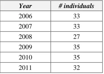
Table S.1. Number of individuals simulated in each baseline year.

Year # individuals

2006 33

2007 33

2008 27

2009 35

2010 35

2011 32

Table S.2. Summary of calf histories. Each calf is associated with the corresponding mother. A calf history is composed of a series of stages, as defined in section 2.2 in the paper. Calf histories have a different length depending on when the calf was born in the period under analysis (2006-2011). Not all 17 modelled females had calves in the period of interest.

Calf ID Mother’s ID Year of birth History

1024 11 2007 1 2 3 3 3

1008 52 2006 1 2 3 3 3 3

1111 52 2010 1 4 4

1020 64 2007 1 2 3 3 3

1010 307 2006 1 2 4 4 4 4

1084 307 2009 1 2 3

1080 430 2008 1 2 3 4

1022 578 2007 1 2 3 3 3

1130 578 2011 1 2

1113 580 2010 1 2

1078 745 2008 1 2 4 4

1012 800 2006 1 2 3 3 3 3

1087 800 2009 1 2 3

1019 820 2007 1 2 4 4 4

1125 820 2011 1 2

1085 866 2009 1 2 3

1110 923 2010 1 2

1086 965 2009 1 2 3

1023 969 2007 1 2 3 3 3

32

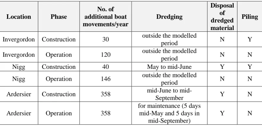
Table S.3. Summary of the activities associated with the construction and operational phases of the three proposed developments. These involve disposal of dredged material and piling, which were not included in the individual-based model.

Location Phase

No. of additional boat movements/year Dredging Disposal of dredged material Piling

Invergordon Construction 30 outside the modelled

period N Y

Invergordon Operation 120 outside the modelled

period N N

Nigg Construction 40 May to mid-June Y Y

Nigg Operation 146 outside the modelled

period N N

Ardersier Construction 358 June to

mid-September Y N

Ardersier Operation 358

for maintenance (5 days mid-May and 5 days in

mid-September)

Y N

Table S.4. Key probabilities estimated from the multi-stage model for calf survival.

Transition probabilities

Probability of calf surviving

the first year 0.87

Probability of calf surviving

to the third year 0.73

Probability of calf surviving

after the third year 0.84 Misclassification probabilities

Probability of misclassifying

a calf at stage 2 as dead 0.05 Probability of misclassifying

a calf at stage 3 as dead 0.05

33

5. Figures

34 a)

35 c)

36 e)

f)

37

38

39

40

41

42

43

44

45

46

6. Detailed acknowledgements

This work received funding from the MASTS pooling initiative (the Marine Alliance for Science and Technology for Scotland) and their support is gratefully acknowledged. MASTS is funded by the Scottish Funding Council (grant reference HR09011) and contributing institutions. The work also benefited from discussions with participants in a working group supported by Office of Naval research grants N00014-09-1-0896 to the University of California, Santa Barbara and N00014-12-1-0274 to the University of California, Davis. Satellite data were received and processed by the NERC Earth Observation Data Acquisition and Analysis Service (NEODAAS) at Dundee University and Plymouth Marine Laboratory (www.neodaas.ac.uk). POLPRED model for tidal information was kindly provided by NERC National Oceanography Centre (Liverpool, UK). Photo-identification data were collected during a series of grants and contracts from the BES, ASAB, Greenpeace

Environmental Trust, Scottish Natural Heritage, Scottish Government, Whale and Dolphin

Conservation, Talisman Energy (UK) Ltd., Department of Energy and Climate Change, Chevron and the Natural Environment Research Council. All survey work was carried out under Scottish Natural Heritage Animal Scientific Licences. We particularly thank Ben Leyshon (Scottish Natural Heritage) for fruitful discussions and support during the development of this project. We thank Tim Barton and all the people that have helped with the data collection. Finally, we would like to thank Len Thomas, Rob Schick, Alex Douglas and Beth Scott for their inputs on the analysis, and Dan Costa and two anonymous reviewers for their useful comments on the manuscript.

7. References

1. Redfern, J. V. et al. 2006 Techniques for cetacean-habitat modeling. Marine Ecology Progress

Series310, 271–295. (doi:10.3354/meps310271)

2. McFarland, D. J. & Sibly, R. M. 1975 The behavioural final common path. Philosophical

Transactions of the Royal Society of London Series B: Biological Sciences270, 265–93.

3. Zucchini, W., Raubenheimer, D. & MacDonald, I. L. 2008 Modeling time series of animal behavior by means of a latent-state model with feedback. Biometrics64, 807–815.

(doi:10.1111/j.1541-0420.2007.00939.x)

4. Frid, A. & Dill, L. 2002 Human-caused disturbance stimuli as a form of predation risk.

Conservation Ecology6, 11.

5. Pirotta, E., Thompson, P. M., Cheney, B., Donovan, C. R. & Lusseau, D. 2015 Estimating spatial, temporal and individual variability in dolphin cumulative exposure to boat traffic using spatially explicit capture-recapture methods. Animal Conservation18, 20–31.

47

6. Pirotta, E., Thompson, P. M., Miller, P. I., Brookes, K. L., Cheney, B., Barton, T. R., Graham, I. M. & Lusseau, D. 2014 Scale-dependent foraging ecology of a marine top predator modelled using passive acoustic data. Functional Ecology28, 206–217. (doi:10.1111/1365-2435.12146) 7. Pirotta, E., Merchant, N. D., Thompson, P. M., Barton, T. R. & Lusseau, D. 2015 Quantifying

the effect of boat disturbance on bottlenose dolphin foraging activity. Biological Conservation

181, 82–89.

8. Lusseau, D., New, L., Donovan, C., Cheney, B., Thompson, P. M., Hastie, G. & Harwood, J. 2011 The development of a framework to understand and predict the population consequences of disturbances for the Moray Firth bottlenose dolphin population. Scottish Natural Heritage Commissioned Report No. 468.

9. New, L. F. et al. 2013 Modeling the biological significance of behavioral change in coastal bottlenose dolphins in response to disturbance. Functional Ecology27, 314–322.

(doi:10.1111/1365-2435.12052)

10. Cheney, B. et al. 2014 Long-term trends in the use of a protected area by small cetaceans in relation to changes in population status. Global Ecology and Conservation2, 118–128. (doi:10.1016/j.gecco.2014.08.010)

11. Wilson, B., Reid, R. J., Grellier, K., Thompson, P. M. & Hammond, P. S. 2004 Considering the temporal when managing the spatial: a population range expansion impacts protected areas-based management for bottlenose dolphins. Animal Conservation7, 331–338. 12. Patterson, T. A., Thomas, L., Wilcox, C., Ovaskainen, O. & Matthiopoulos, J. 2008

State-space models of individual animal movement. Trends in Ecology & Evolution23, 87–94. (doi:10.1016/j.tree.2007.10.009)

13. Dellaportas, P., Forster, J. & Ntzoufras, I. 2002 On Bayesian model and variable selection using MCMC. Statistics and Computing12, 27–36.

14. Kuo, L. & Mallick, B. 1998 Variable selection for regression models. Sankhyā: The Indian

Journal of Statistics, Series B, 1–17.

15. Wood, S. N. 2006 Generalized additive models, an introduction with R. Chapman & Hall/CRC, London.

16. R Development Core Team 2013 R: A language and environment for statistical computing. R Foundation for Statistical Computing, Vienna, Austria. ISBN 3-900051-07-0, URL

http://www.R-project.org/.