Coupling Interactions and Trapped Effects for a
Triple-Well Potential
Sezgin Aydın, Mehmet Şimşek
Department of Physics, Faculty of Sciences, Gazi University, Ankara, Turkey E-mail: [email protected]
Received March 24, 2011; revised May 6, 2011; accepted May 20, 2011
Abstract
Weak and strong coupling interactions and trapped effects have always played a significant role in under-standing physical and chemical properties of materials. Triple-well anharmonic potential may be modeled for interpretation of energy spectra from the nuclear to macro molecular systems, and also crystalline systems. Exact periods of a trapped particle in each well of the potential are explicitly derived. For the extended Duffing system, it is predicted that infinite series of both frequency and spatial trajectory approach to exact results in the limit of weak-coupling cases (g→0).
Keywords: Perturbation Method, Triple-Well Potential, Duffing Equation, Weak and Strong Couplings.
1. Introduction
The physics of nonlinear systems is one of the important research interests in both quantum and classical mechan-ics, and its oscillatory representation [1-7] occupies spe-cial place for dynamical systems. There are different kinds of nonlinear oscillator problems that arise in the study of dynamical systems. In that, the extension of well-known nonlinear pendulum theory to the one di-mensional oscillator model has been widely used to si-mulate classical and quantum systems (see some of ref-erences [1-17]).
Nonlinear oscillatory systems are widely used tools for the modeling of atomic, molecular and crystalline sys-tems [12-23]. Although overall reliability of the quantum and classical interpretations is controversial, the simple theoretical correspondence and appropriate calculations make them popular, among the theoretically physicists and chemists [19-25]. Now, let us consider a second or-der one dimensional anharmonic oscillator equation,
3
5
0x t cx t g x t ax t
(1)
with the arbitrary parameters of c, g and a. Note that if the parameters in the equation are chosen as c = w02, g =
–1/6 w02 and a = –1/20, it turns to fifth order non-linear
equation of elementary (1+1) dimensionally pendulum, and also to the Duffing equation [26-28] for a = 0. How- ever, using the perturbation approximations [21], a mod-el of nonlinear problem, other words the extended
Duff-ing equation, reduces to approximately solvable case. So, we called it here after the extended Duffing oscillator.
It is important that the range of applicability of this equation is fairly wide than that of Duffing oscillator, and in particular, it includes extra free parameter (a). Other words, the arbitrary parameters (i.e., g and a) stand for the perturbation parameter and coupling constants for weak-coupling systems, respectively. It may be modeled for coherent tunneling via adiabatic passage in a triple- well system and coherent transport of electrons between quantum dots or atoms in micro-magnetic traps [18]. Generally, for weak-coupling systems, anharmonic terms can be treated as a perturbation, that well-known first detailed example is quartic anharmonic potential by Bender and Wu [24, 25]. By our assumptions, in order to parallel analysis, this new nonlinear equation may be called Duffing+ax5 equation.
Let us integrate the dynamical system in Equation (1) with respect to time,
px,
2 2 2 4 6
0
1 1 1 1
2p t 2w x t 4gx t 6agx t E (2) where the integral constant E (Energy) can be imposed in terms of the potential parameters. By using the initial conditions for frequency (w0) and location (x0) at t = 0,
and also for the parameters a and g, it can be settled as,
2 2 4 6
0 0 0 0
S. AYDIN ET AL. 899
So, the reducible potential in Equation (2) can be written as,
2 2
4
6
0
1 1 1
2 4 6
V x w x t gx t agx t (3)
which has different shapes, as a modeling of systems, for given potential parameters w0, a and g (see Figure 1).
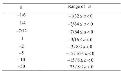
[image:2.595.317.526.117.239.2]Note that, if one wants to get the special shapes of the potential, such as one and two or three wells, the restric-tions must be constructed among the parameters as in Table 1, which shows the possible range of the potential parameters for triple-well behavior.
On the other hand, for given initial energy (E) and ini-tial parameters, dynamical equation of the system in Eq-uation (2) can be written as,
px,
2 3 5
0
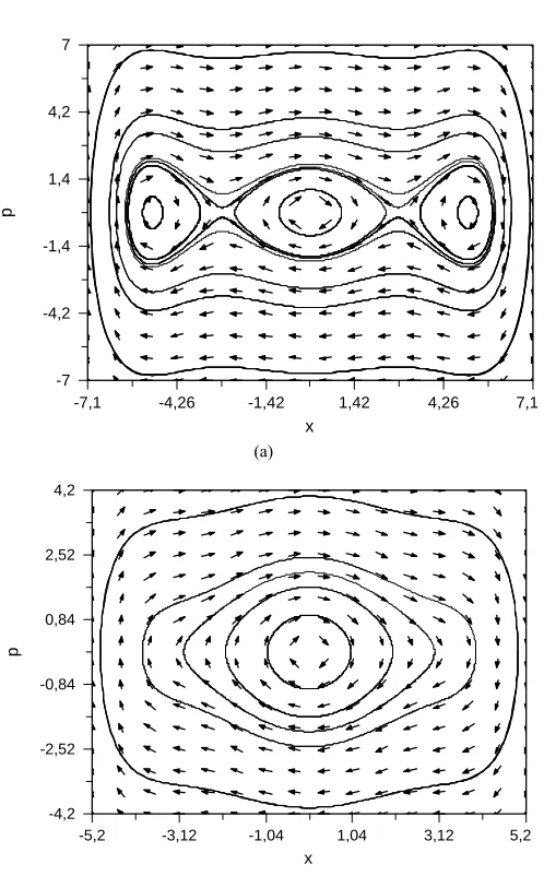
p w x g x ax (4) For chosen g and a parameters, which they are gene-rating three-well and one-well potentials, phase portraits are shown in Figures 2 (a) and (b), respectively. It is seen that the closed orbits are for bonded cases in the trajecto-ries, are correspond different potential shapes. However, both of bounded (closed orbits) and unbounded cases (open orbits) can be situated, i.e., all initial conditions could not lead to the stable equilibrium points and closed orbits. Other words, the image of a periodic solution in the phase portrait is a closed trajectory that is usually called periodic orbit also. Therefore, instead of trying to
Table 1. The range of the parameter a for given some g values of triple-well potentials in the interval
( 50 g 1/ 6)
g Range of a
–1/6 1 32 a 0 –1/4 3 64 a 0 –7/12 7 64 a 0 –1 3 16 a 0 –2 3 / 8 a 0 –5 15 /16 a 0 –10 15 / 8 a 0 –50 75 / 8 a 0
solve the equation for all phase paths, we would like to find the periodic solutions as
2π/
x t x t w (5)
for the bonded cases, with the initial conditions,
0 1x , x
0 0 (6)By our initial assumptions, we apply the Lindstedt- Poincaré perturbation method [26-28] to the non-linear Duffing + ax5 oscillatory system, in following section
[image:2.595.141.454.424.689.2](Section 2). In Section 3, we derive the exact quarter periods expressions for a particle in the triple-well poten-tial. Hence, we calculate the weak and strong interaction
-7,1 -4,26 -1,42 1,42 4,26 7,1 x
-7 -4,2 -1,4 1,4 4,2 7
p
(a)
-5,2 -3,12 -1,04 1,04 3,12 5,2
x
-4,2 -2,52 -0,84 0,84 2,52 4,2
p
[image:3.595.177.426.66.467.2](b)
Figure 2. The phase portraits of sextic anharmonic oscillator potential with fixed g = –1/6 and different values of anharmo-nicity parameter a; a) for tree-finite gap cases, a = –3/100; and b) for one-finite gap cases, a = –5/100. The values of the para-meters chosen as the corresponding coefficients of the Taylor expansion of sin(θ).
limit cases for the purposed system in Sec.4. Finally, the paper ends with discussion section Sec.5.
2. Weak-Coupling Interactions
Classical Lindstedt-Poincaré approach [26-28], it’s mod-ified version [23, 29-30] and also linear delta expansion method [31] are powerful methods for generating peri-odic perturbation series of the non-linear anharmonic oscillatory systems. We now consider rescale time ac-cording to
wt
( )
q x
w
(7)
then, Equation (1) can be written as
2 2 3 5
0
( ) ( ) ( ) ( ) 0,
w q w q g q aq (8)
with the initial conditions, (0)q x0, (0) 0q , where,
the prime denotes differentiation with respect to new time variable, ξ. Thus, the periodicity is
( ) ( 2π)
q q for new variables. The fact that
peri-odic solutions of equations can be expressed as an infi-nite series [23] for small coupling parameter
( 2 2
0/ 0
gw x ),
2 0
0 2
0 0
( ) ( )
n
n n
x g
q q w
w
(9)and also, frequency w can be expanded as
2 0
0 2
0 0
n
n n
x g
w w w
w
(10)S. AYDIN ET AL. 901
perturbation parameter g, it can be obtained a recursive
set of simple ordinary differential equations: qn( ) qn( ) fn( ), qn(0) qn(0) 0
(11)
where
1 1 1 1
0 1
1 1 1 0 0
1 1
1 1
1
0 0 0 0
( ) 2 ( ) 2 ( ) ( ) ( ) ( ) ( )
, 1, 2,3,...
n n n m n n m
n n l n l m l n m l m l n m l
l m l m l
n i j n i j k n n i
i j k l n i j k l
i j k l
f w q w q w w q q q q
a q q q q q n
(12)without impairing the generality, we can impose initial values: w0 = 1 and x0 = 1. The initial trajectory could be
chosen as q0( ) cos( ) . Otherwise, fn( ) functions can be expanded to a Fourier series
2 , 0
( ) n ( ) cos (2 1)
n n k
k
f f a k
(13)with starting coefficients as fn,0 = 0. Note that choosing
of this initial value, the secular terms in the solutions of Equation (11) are vanish. On the other hand, we can write
2 , 2 1 ( )( ) ( ) cos( ) cos[(2 1) ]
1 2 1
n n k
n n
k
f a
q l a k
k
(14)where
2 1 ,2 , 2 2 1 ( ) ( )4 1 1 1 2 1
n
n n n k
n
k
f f a
l a
n k
(15) Note that, these general expressions can be predicted analytically using simple algebra. Substituting general definitions (12-13) in differential Equation (11), we find the corresponding series forw a g( , ) and x w a g t( , , ; )(Equations (9) and (10)),
2
2 3
3 5 21 19 215
( , ) 1 ( )
8 16 256 128 3072
a a a
w a g g g O g
(16)
1 5 1
( , , ; ) cos( ) cos( ) cos(3 ) cos(5 )
32 24 128 32 384
a a a
x w a g t wt wt wt wt g
2 2
23 605 3791 3 205 5
cos( ) cos(3 )
1024 12288 147456 128 4096 192
a a a a
wt wt 2 2 2 3
1 7 95
cos(5 ) cos(7 ) cos(9 ) ( )
1024 12288 4096 294912 98304
a a a a
wt wt wt g O g
(17)
It is note that, these infinity series of w(a,g) approach the exact results in the limit g→0 for the weak-coupling systems and, the series of trajectory x(w,a,g;t) coincide with the fourth-order Runge-Kutta method results. On the other hand, it is seen that when a is choosed as zero, this formulation is reduced to solution of well-known Duffing oscillator [9-11,23,26-28]. However, fn,k(a) and ln(a) functions are listed in Tables 2 and 3, respectively.
3. Exact Solutions of a Particle in the
Triple-Well Potential
Classically, it is simple to combine time and space va-riables under certain conditions. Substituting p (from Equation (4)), it can be integrated over a quarter period. Thus, we obtain exact quarter period for a particle in the triple-well potential as
0
0 2 2 2 2
0 1 2
d 2
3
x
x
w ag x x x u x u
(18)where 02 1 3 2 4 x u G a
, and
2 0 2 3 2 4 x u G a ,
with
2 2 2 4
0 0 0
3 3 / 16 / ( ) 4 / 4
4
a w ag x a x
G .
Changing the variable x2 = y, period integral turns to
2 0
2
0 0 1 2
π 1 3 d
2 2
x
y
w ag
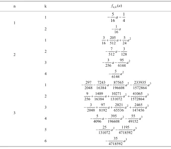
y x y y u y u (19)Table 2. The coefficients of inhomogeneous oscillatory equations, fn k, ( )a , of weak coupling cases (n3) in Equation (13).
Coefficients were computed using Equation (13).
n k fn k, ( )a
1
1 5 1
16a 4
2 1
16a
2
1 3 205 5 2
16 512 a24a
2 7 3
512a 128
3 3 95 2
256a 6144a
4 5 2
6144a
3
1 297 7243 87565 2 233935 3 2048 16384a 196608a 1572864a
2 9 1409 10271 2 41065 3
256 16384 a131072a 1572864a
3 3 97 2021 2 2465 3
2048 8192a 65536a 147456a
4 5 395 2 55 3
4096a 196608a 49152a
5 25 2 1195 3
131072a 4718592a
6 35 3
4718592a
Table 3. The coefficients of the solutions of weak coupling cases (n4) in Equation (14), which were calculated using Equa-tion (15). Coefficients depend on coupling parameter a.
n l an( )
1 1 1
32 24a
2 23 605 3791 2
1024 12288 a147456a
3 547 6743 81461 2 60769 3
32768 131072a 1572864a 3538944a
4 6713 322145 3829667 2 181124033 3 1067484605 4
524288 6291456 a50331648a 3623878656a 86973087744a
of potential parameters leads to different varieties of po-tential shapes and equilibrium conditions. Therefore, having defined equilibrium points, our task now is to find period of trapped particle in one of potential wells:
1) At middle well: choosing the parameters as,
2
2, , , , 1 0 0
a u b u c x u c d , and then using the equation (3.147.2) in Ref. [32],
2 0
2
0 0 1 2
1 3 d
2 2
x
y
w ag y x y y u y u
(20)we can find the exact quarter period as
2
2 1 0
2 2
2 0 1
2 0 1
3 1
,
2 2
u u x
F
w ag u x u u x u
(21)
where F( , ) k is elliptic integral of the first kind [32]
2 2
0
d ( , )
1 sin ( )
F k
k
(22)S. AYDIN ET AL. 903
as 2
2, , , , 01 0
a u c u b x u a d , and then, we use the equation (3.147.6) in Ref. [32],
2
2 0
2
0 1 2
π 1 3 d
2
u
x
y
w ag
y x y y u y u (23)Thus, we can find exact half period of particle with positive energy as
2
2 0 1
2 2
2 1 0
2 1 0
π 3 1 π
, 2
u x u
F
w ag u u x u u x
(24)
On the other hand, if the particle has negative energy and in right (or left) well, we set the parameters as:
2
2, 0, 0, , 1
a u c b x u a d u , and then using equ-ation (3.147.6) in Ref.[32],
2
2 0
2
0 1 2
π 1 3 d
2
u
x
y
w ag
y x y y u y u (25)we can find the exact half period as
2
2 0 1
2 2
0 1 2
0 1 2
π 3 1 π,
w 2
u x u
F
ag x u u x u u
(26)
It is note that, if we expand Equation (21) for limit (g→0), as expected for weak coupling cases, there is an excellent agreement between expansion and Equation (16), i.e., they are the same.
4. Strong-Coupling Limit
Let us rewrite Equation (21), for middle range, as
22 2 0
0
π 1 3 1
3 3 16 / 4 4
2 ( ) 4 2 12
w a
w g w a g a a
K r g
(27)
where K(r)=F(/2, r) is elliptic K function, (8.112.1) in Ref.[32],. The new variable is r 2 / with
2
3 3g g 4a g 16a 4ag
,
12 9g 6ag ,
respectively . Our purpose is to find the series expansion of the periods in large asymptotic limit, g→∞. Hence, we can write frequency series as,
2
2 2 2
0 0 0
0 1 2 , ( )
n
n
w w w
w g b b b b g
g g g
(28)
where first three coefficients are
0
2
π
4 3
b
(29)
and,
1
3 2 3
2 π 3 2
2 a
a
b a
(30)
2 2 32 3 2 2 2 2 2
7 6 5 3 4 4 3 3 3
2 3 2 2
2
12 2 9 6
π 2 576 288 2
3 16 2
82944 290304 228096 1152 134784 1152 12416
2
1728 2592
46656
a a a
a a
a a
b
a
a a a a a a a
a a a
with the abbreviations
2
9 12a 12a
, 9 6a, 3 2a ,
3 6a
, 2 2 EllipticK , 2 2 EllipticE
2 2 1 , 2 1 , a
144a 216
a , 3/ 2
1 96 128
2a 1
4 2 2 a
respectively.
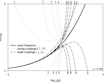
In order to compare, we figure out the weak-coupling and strong-coupling expansions together with the exact result in Figure 3. It can be indicated that the curve of exact result is appearing as a ‘cut line’ between last term of the expansions odd and even order for two different classes of interactions. In the other words, if the order of last term of expansion is even (odd) then, corresponding curve lies below (above) the curve of exact results. Note that the plot of extended Duffing systems is similar to that of the Duffing systems (see Figure 1 in Ref. [23]). In Figure 4, we plot of weak-coupling perturbation se-ries (10) versus to the coupling parameter a for fixed g = –1/6, where corresponding perturbation orders are marked in label (1 - 11). It should also be noted that, as expected for weak-coupling cases, the convergence rate increases while value of a decreases (see Figure 4).
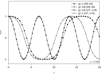
In addition to the Duffing systems, a more general sit-uation has been investigated for the Duffing and Duff-ing+ax5 dynamical systems. On the other hand, we also
solve the equation by numerical Runge-Kutta (RK) me-thod that, the solutions coincide with LP profiles only in small absolute value of parameter g (|g|<1). The results
are shown in Figure 5, where we plot spatial profile of oscillator versus time. These results are interesting not only in the convergence of both dynamical properties but also in the context of realistic physical systems. It is shown that period of system increases, while the absolute value of parameter g decreases.
5. Conclusions
We have shown that dynamical solutions of the extended Duffing oscillator, the corresponding to the family of quantum triple-well potentials can be closely approx-imated by choosing appropriate potential parameters. The basic advantages of the approach are due to its spe-cific properties of quantum triple-well oscillator potential. We can say that our algorithm is more flexible for other polynomial potentials, and also reproduces infinite per-turbation series for the trajectories and the frequencies of a trapped particle within limit of weak and strong coupl-ing interactions. Of course, weak and strong couplcoupl-ing interactions and the trapped effects are important inmany fields of physics such as particle physics, atomic, mole-cular and macromolemole-cular systems. It should be re-marked that, there is a good agreement between the
log10(g)
-1 1
w
(
a
,g
)
1 2
exact frequency strong couplings weak couplings
a=-3/100
1
2 3
4 5
6 7
8 9
1
2
3
4
5
6 7
8 9
( 1...9 )
1 9
[image:7.595.122.480.383.668.2]( ... )
S. AYDIN ET AL. 905
a
-10 -8 -6 -4
w(
a,g)
1,2 1,3 1,4
g=-1/6
1
2 3
4 5
6
7
8 9
[image:8.595.134.463.78.373.2]10 11
Figure 4. The plot of weak-coupling perturbation series (10) versus parameter a for middle range (for fixed g = –1/6). The numbers at the figure indicate that the order of perturbation series.
t
0 5 10 15 20
x(t
)
-1 0 1
g=-1 (RK 45) g=-1/6 (RK 45) g=-1/6 (LP, n=8) g=-1 (LP, n=8)
a=-3/100
[image:8.595.121.470.417.674.2]results of the Lindstedt-Poincaré perturbation method and our analytic results for weak coupling cases.
6. References
[1] J. H. He, “An Elementary Introduction to Recently De-veloped Asymptotic Methods and Nanomechanics in Textile Engineering,” International Journal of Modern Physics B, Vol. 22, No. 21, 2008, pp. 3487-3578.
doi:10.1142/S0217979208048668
[2] F. M. Fernandez and R. H. Tipping, “Accurate Calcula-tion of VibraCalcula-tional Resonances by PerturbaCalcula-tion Theory,” Journal of Molecular Structure (Theochem), Vol. 488, No. 1-3, 1999, pp. 157-161.
doi:10.1016/S0166-1280(98)00622-8
[3] F. J. Gomez and J. Sesma, “Bound States and “Reson-ances” in Quantum Anharmonic Oscillators,” Physics Letters A, Vol. 270, No. 1-2, 2000, pp. 20-26.
doi:10.1016/S0375-9601(00)00290-5
[4] A. Pathak and S. Mandal, “Classical and Quantum Oscil-lators of Quartic Anharmonicities: Second-Order Solu-tion,” Physics Letters A, Vol. 286, No. 4, 2001, pp. 261-276. doi:10.1016/S0375-9601(01)00401-7
[5] A. Pathak and S. Mandal, “Classical and Quantum Oscil-lators of Sextic and Octic Anharmonicities,” Physics Let-ters A, Vol. 298, No. 4, 2002, pp. 259-270.
doi:10.1016/S0375-9601(02)00500-5
[6] Y. Meurice, “Arbitrarily Accurate Eigenvalues for One-Dimensional Polynomial Potentials,” Journal of Physics A: Mathematical and General, Vol. 35, No. 41, 2002, pp. 8831-8846.
doi:10.1088/0305-4470/35/41/314
[7] I. A. Ivanov, “Transformation of the Asymptotic Pertur-bation Expansion for the Anharmonic Oscillator into a Convergent Expansion,” Physics Letters A, Vol. 322, No. 3-4, 2004, pp. 194-204.
doi:10.1016/j.physleta.2004.01.014
[8] H. K. Khalil, “Nonlinear Systems,” Maxwell Macmillan, Toronto, 1992.
[9] J. H. He, “Some New Approaches to Duffing Equation with Strongly and High Order Nonlinearity (II) Parame-trized Perturbation Technique,” Communications in Non-linear Science and Numerical Simulation, Vol. 4, No. 1, 1999, pp. 81-83. doi:10.1016/S1007-5704(99)90065-5
[10] J. Lin, “A New Approach to Duffing Equation with Strong and High Order Nonlinearity,” Communications in Nonlinear Science and Numerical Simulation, Vol. 4, No. 2, 1999, pp. 132-135.
doi:10.1016/S1007-5704(99)90026-6
[11] J. H. He, “Variational Iteration Method—a Kind of Non-Linear Analytical Technique: Some Examples,” In-ternational Journal of Non-Linear Mechanics, Vol. 34, No. 4, 1999, pp. 699-708.
doi:10.1016/S0020-7462(98)00048-1
[12] Y. Z. Chen, “Solution of the Duffing Equation by Using Target Function Method,” Journal of Sound and Vibra-tion, Vol. 256, No. 3, 2002, pp. 573-578.
doi:10.1006/jsvi.2001.4221
[13] A. R. Chouikha, “Series Solutions of Some Anharmonic Motion Equations,” Journal of Mathematical Analysis and Applications, Vol. 272, No. 1, 2002, pp. 79-88.
doi:10.1016/S0022-247X(02)00134-8
[14] M. El-Kady and E. M. E. Elbarbary, “A Chebyshev Ex-pansion Method for Solving Nonlinear Optimal Control Problems,” Applied Mathematics and Computation, Vol. 129, No. 2-3, 2002, pp. 171-182.
doi:10.1016/S0096-3003(01)00104-7
[15] C. W. Lim and B. S. Wu, “A New Analytical Approach to the Duffing-Harmonic Oscillator,” Physics Letters A, Vol. 311, No. 4-5, 2003, pp. 365-373.
doi:10.1016/S0375-9601(03)00513-9
[16] Y. Z. Chen, “Evaluation of Motion of the Duffing Equa-tion from Its General Properties,” Journal of Sound and Vibration, Vol. 264, No. 2, 2003, pp. 491-497.
doi:10.1016/S0022-460X(02)01495-5
[17] H. R. Marzban and M. Razzaghi, “Numerical Solution of the Controlled Duffing Oscillator by Hybrid Functions,” Applied Mathematics and Computation, Vol. 140, No. 2-3, 2003, pp. 179-190.
doi:10.1016/S0096-3003(02)00112-1
[18] T. Opatrný and K. K. Das, “Conditions for Vanishing Central-Well Population in Triple-Well Adiabatic Trans-port,” Physics Letters A, Vol. 79, No. 1, 2009, p. 02113. [19] V. B. Mandelzweig and F. Tabakin, “Quasilinearization
Approach to Nonlinear Problems in Physics with Appli-cation to Nonlinear ODEs,” Computer Physics Commu-nications, Vol. 141, No. 2, 2001, pp. 268-281.
doi:10.1016/S0010-4655(01)00415-5
[20] J. I. Ramos, “Linearization Methods in Classical and Quantum Mechanics,” Computer Physics Communica-tions, Vol. 153, No. 2, 2003, pp. 199-208.
doi:10.1016/S0010-4655(03)00226-1
[21] J. L. Trueba, J. P. Baltanas and M. A. F. Sanjuan, “A generalized Perturbed Pendulum,” Chaos, Solitons & Fractals, Vol. 15, No. 5, 2003, pp. 911-924.
doi:10.1016/S0960-0779(02)00210-2
[22] A. Post and W. Stuiver, “Modeling Non-Linear Oscilla-tors: A New Approach,” International Journal of Non- Linear Mechanics, Vol. 39, No. 6, 2004, pp. 897-908.
doi:10.1016/S0020-7462(03)00073-8
[23] A. Pelster, H. Kleinert and M. Schanz, “High-Order Var-iational Calculation for the Frequency of Time-Periodic Solutions,” Physical Review E, Vol. 67, No. 1, 2003, p. 016604. doi:10.1103/PhysRevE.67.016604
[24] C. M. Bender and T. T. Wu, “Analytic Structure of Energy Levels in a Field-Theory Model,” Physical Re-view Letters, Vol. 21, No. 6, 1968, pp. 406-409.
doi:10.1103/PhysRevLett.21.406
[25] C. M. Bender and T. T. Wu, “Anharmonic Oscillator,” Physical Review, Vol. 184, No. 5, 1969, pp. 1231-1260.
doi:10.1103/PhysRev.184.1231
S. AYDIN ET AL. 907
[27] N. Minorsky, “Nonlinear Oscillation,” Van Nostrand, Princeton, 1962.
[28] A. H. Nayfeh, “Introduction to Perturbation Techniques,” John Wiley, New York, 1981.
[29] J. H. He, “Modified Lindstedt–Poincare Methods for Some Strongly Non-Linear Oscillations: Part I: Expan-sion of a Constant,” International Journal of Non-Linear Mechanics, Vol. 37, No. 2, 2002, pp. 309-314.
doi:10.1016/S0020-7462(00)00116-5
[30] J. H. He, “Modified Lindstedt–Poincare Methods for Some Strongly Non-Linear Oscillations: Part II: A New
Transformation,” International Journal of Non-Linear Mechanics, Vol. 37, No. 2, 2002, pp. 315-320.
doi:10.1016/S0020-7462(00)00117-7
[31] P. Amore and A. Aranda, “Presenting a New Method for the Solution of Nonlinear Problems,” Physics Letters A, Vol. 316, No. 3-4, 2003, pp. 218-225.
doi:10.1016/j.physleta.2003.08.001