Crowdsourced Sampling of a Composite Random Variable: Analysis, Simulation, and Experimental Test

(1)

ISSN Online: 2161-7198 ISSN Print: 2161-718X

DOI: 10.4236/ojs.2019.94034 Aug. 15, 2019 494 Open Journal of Statistics

Crowdsourced Sampling of a Composite

Random Variable: Analysis, Simulation,

and Experimental Test

M. P. Silverman

Department of Physics, Trinity College, Hartford, CT, USA

Abstract

A composite random variable is a product (or sum of products) of statistically distributed quantities. Such a variable can represent the solution to a mul-ti-factor quantitative problem submitted to a large, diverse, independent, anonymous group of non-expert respondents (the “crowd”). The objective of this research is to examine the statistical distribution of solutions from a large crowd to a quantitative problem involving image analysis and object count-ing. Theoretical analysis by the author, covering a range of conditions and types of factor variables, predicts that composite random variables are distri-buted log-normally to an excellent approximation. If the factors in a problem are themselves distributed log-normally, then their product is rigorously log-normal. A crowdsourcing experiment devised by the author and imple-mented with the assistance of a BBC (British Broadcasting Corporation) tele-vision show, yielded a sample of approximately 2000 responses consistent with a log-normal distribution. The sample mean was within ~12% of the true count. However, a Monte Carlo simulation (MCS) of the experiment, employing either normal or log-normal random variables as factors to model the processes by which a crowd of 1 million might arrive at their estimates, resulted in a visually perfect log-normal distribution with a mean response within ~5% of the true count. The results of this research suggest that a well-modeled MCS, by simulating a sample of responses from a large, ration-al, and incentivized crowd, can provide a more accurate solution to a quantit-ative problem than might be attainable by direct sampling of a smaller crowd or an uninformed crowd, irrespective of size, that guesses randomly.

Keywords

Crowdsourcing, Computer Modeling of Crowds, Monte Carlo Simulation, Large-Scale Sampling, Log-Normal Random Variable, Log-Normal How to cite this paper: Silverman, M.P.

(2019) Crowdsourced Sampling of a Com-posite Random Variable: Analysis, Simula-tion, and Experimental Test. Open Journal of Statistics, 9, 494-529.

https://doi.org/10.4236/ojs.2019.94034 Received: July 12, 2019

Accepted: August 12, 2019 Published: August 15, 2019 Copyright © 2019 by author(s) and Scientific Research Publishing Inc. This work is licensed under the Creative Commons Attribution International License (CC BY 4.0).

http://creativecommons.org/licenses/by/4.0/

(2)

DOI: 10.4236/ojs.2019.94034 495 Open Journal of Statistics

Distribution

1. Introduction: Estimation of an Unknown Composite

Quantity by Large-Scale Sampling

The global reach of telecommunications media, including radio, television, and in particular the social media sites of the internet, make possible an ease and scale of statistical sampling hitherto inconceivable. Through use of these media, almost any question can, at least in principle, be posed to a large, anonymous, diverse, independent population of respondents, referred to in both technical and non-technical literature as the “crowd” [1]. This paper reports a compre-hensive 1) analytical investigation, 2) Monte-Carlo simulation, and 3) experi-mental test of the distribution of a composite random variable (RV) representing a crowdsourced response to a question calling for a numerical answer. A com-posite RV is a product of two or more factor RVs. In the following sections it is shown that:

1) the most useful characteristic of a crowdsourced sample is its distribution function and not just a single statistic,

2) under conditions to be specified, a product of RVs is distributed log-normally to an excellent approximation, irrespective of the type or number or correlation of factor RVs,

3) computer simulation methods can model the response of a hypothetical ra-tional crowd orders of magnitude larger than what actually might be practically attainable.

1.1. Background

To the author’s knowledge, the first quantitative experiment in what today would be considered crowdsourcing was published by the English polymath and statistical innovator Sir Francis Galton in 1907 [2] [3]. Galton collected all the estimates of the weight of a dressed ox (i.e. the carcass weight) submitted by contestants at the annual West of England Fat Stock and Poultry Exhibition. To his surprise, he found that the sample median of 1207 pounds differed from the measured weight of 1198 pounds by a mere +0.8% and that the sample mean of 1197 pounds differed by an even smaller fractional error of −0.08%. The sample size was reported to be about 800. There was no mention of the sample distribu-tion.

(3)

in-DOI: 10.4236/ojs.2019.94034 496 Open Journal of Statistics

vestigated recently are questions regarding methods of sampling, quality control, bias elimination, and effectiveness [6] [7] [8] [9].

This paper addresses a different aspect of crowdsourcing closer in nature to the kind of experiment first performed by Galton. Questions whose responses can be represented numerically are especially suitable for statistical analysis. In this regard, the most useful statistical information to obtain from a crowd-sourced sample is its distribution—i.e. the probability function for a discrete random variable (RV), or probability density function (PDF) for a continuous RV, or cumulative distribution function (CDF) for either kind of RV. For sim-plicity of discussion, the designation PDF will apply here to both discrete and continuous RVs. The importance of knowing the PDF or CDF of a distribution is that one can calculate from it, either theoretically or numerically, the exact population moments, which, depending on the size of an actual sample, can be significantly different from the sample moments. The population moments are estimates of the statistics that would result from a hypothetical infinitely large population of independent respondents. A virtually infinite sample size is what the internet and mass media have the potential to provide; it is also what com-puter-based Monte Carlo simulation (MCS) methods are already able to provide.

Throughout the past two decades, the author has conducted an array of expe-riments with students in his physics courses to investigate the validity of the crowdsourcing hypothesis [10]. In particular, tests were designed to examine whether groups of non-experts excelled over specialists in exercises relating to estimation, prediction, and deduction. Because sample sizes were relatively small (below 100), histograms of responses showed significant fluctuations, and the results did not appear to be accounted for by a universally applicable distribu-tion. However, a larger-scale experiment (discussed in Section 4) to test crowd-sourced sampling, implemented with the collaboration of a BBC One television show, yielded preliminary results that strongly suggested a log-normal distribu-tion of estimates [10]. The present paper is the outcome of a more general and thorough analysis to extract information contained in a crowdsourced sample.

This paper reports a comprehensive study of the distribution of responses to a class of questions that calls for estimation of a composite random variable. A composite RV is formed by the product of two or more basis RVs. (The term “composite” is adopted from the designation of a “composite number” [11] as an integer expressible as the product of two or more integers, in contrast to a prime number.) This type of question is widely applicable to problems involving ma-thematics, statistics, physical sciences, engineering, bio-medical sciences, foren-sics, business and finance, military science, political science, archaeology, and other fields dependent upon quantitative reasoning.

(4)

high-energy physicists may enlist a crowd to count events recorded in a complex bubble-chamber image; astronomers may enlist a crowd to search a deep-space image for some extraordinary astrophysical event or object; intelligence services may enlist a crowd to search reconnaissance images for locations or objects of military interest, archaeologists may enlist a crowd to search satellite images for structures associated with some cultural sites, and so on [12] [13] [14] [15] [16]. The specific problem examined in this paper is mathematically simple, but statistically informative: How many identical opaque objects are contained within a certain 3-dimensional volume of space seen only as a 2-dimensional image? The problem involves image analysis and object counting. A reasonable procedure to answer that question might entail the following: 1) Depending on the shape of the region, multiply together the appropriate geometric factors to obtain the volume, and then 2) multiply that volume by the numerical density,

i.e. the number of objects in a unit volume. However, none of the needed num-bers is known; all are representable by random variables whose realizations (i.e. estimates) by respondents in the crowd would be different. The sought-for RV would, in general, be a product (or sum of products) of 3 RVs relating to geome-try and 1 RV characterizing the numerical density—or in all a product (or sum of products) of 4 RVs. The analyst is then faced with three general questions:

1) How are the basis RVs distributed?

2) What will be the distribution of the composite RV?

3) Which statistic of the composite RV should be taken to represent the phys-ical value of the sought-for quantity?

By examining this archetypical question a) theoretically, b) computationally by Monte Carlo simulation, and c) experimentally, this paper addresses the pre-ceding three questions.

1.2. Organization

The remainder of this paper is organized in the following way:

Section 2 investigates analytically the distribution of a composite random va-riable comprising independent basis RVs. Of particular interest are the cases in which the basis is either normally or log-normally distributed.

Section 3 investigates numerically by MCS the distributions of a composite variable comprising basis RVs whose distributions differ widely in shape para-meters (skewness, kurtosis) for fixed location and scale parapara-meters (mean, va-riance).

Section 4 reports 1) an experiment, implemented with the collaboration of a British national television show, to employ crowdsourcing as a means to esti-mate the number of opaque objects in a transparent receptacle, and 2) the use of MCS to predict the statistical results for a hypothetical much larger crowd in-centivized to estimate rationally rather than guess randomly.

Section 5 concludes the paper with a summary of principal findings.

(5)

are listed below in alphabetical order. BBC = British Broadcasting Corporation CDF = cumulative distribution function CF = characteristic function

CLT = central limit theorem MCS = Monte Carlo simulation(s) MGF = moment generating function PDF = probability density function RNG = random number generator RV = random variable

2. Distribution of a Composite Random Variable

2.1. General Case

Consider a random variable Z defined by the product

(

)

1 , N

i i i i

Z X

µ σ

=

∏

₍₁₎

where each basis variable Xi

(

µ σi, i

)

in Equation (1) is characterized by its

mean µi and standard deviation σi. At this point, the symbol X represents an arbitrary RV, and the parameters

(

µ σi, i

)

for defining Xi were chosen to simplify the notation and analysis in sections to follow. Conventional statistical labeling of specific RVs that are relevant to this paper may include parameters different from the mean and standard deviation, as summarized in Table 1. The symbol H x

( )

employed in Table 1 is the Heaviside function, also known as the step function, which we define here as

( )

1₀ x 0₀

H x

x

≥  =  _<

 (2)

(There are different definitions of H x

( )

depending on the value assigned to

( )

0

[image:5.595.211.534.575.728.2]

H [17].) A statistical convention followed in this paper is to represent a random variable by an upper case letter, e.g. X, and a variate (i.e. sample or rea-lization of the random variable) by a corresponding lower case letter, e.g. x.

Table 1. Representation of relevant random variables. Distribution of

RV X Representation Symbolic of Parameters Significance PDF normal or

Gaussian N

(

µ σ, 2

)

mean of

standard deviation of X X µ σ = =

( )2 2 1 exp 2 2π x µ σ σ  −  −      

log-normal _Λ

(

_{m s}_, 2

)

mean of ln( )

standard deviation of

m Y X

s Y

= =

=

( )

(

)

2 2 ln 1 _exp 2 2π x x µ σ σ  ₋  −     

uniform U a b

( )

, lower boundary

upper boundary a

b =

= b a−1 H x a( − )−H x b( − )

Laplace La

(

µ β,

)

location parameter

scale parameter

µ β

=

= 21 exp

(6)

The natural logarithm of Z, which is a more convenient RV to work with, takes the form

( )

1

ln N ln i

i

Y Z X

=

= =

∑

_{. (3)}

Reciprocally, one can write

( )

exp

Z = Y . (4) The strategy of the analysis in this section is to calculate the mo-ment-generating function (MGF) of Y defined by the expectation operation

( )

exp

( )

eyt

( )

d

Y Y

g t ≡ Yt =

_∫

p y y₍₅₎

in which p yY

( )

is the PDF of Y, and t is a dummy variable the differentiation

of which generates the statistical moments

k

=

0,1,2,



in the following way:

( )

₀

d d

k k k

Y _t

Y _{= } g t t _₌ _{. (6)}

If the MGF of a random variable does not exist, one can always use the cha-racteristic function (CF) defined by

( )

exp

( )

eiyt

( )

d

Y Y

h t ≡ iYt =

_∫

p y y₍₇₎

where Equation (7) is recognized as the Fourier transform of p yY

( )

[18]. Each

random variable is uniquely characterized by its MGF (if it exists) and CF [19]. By identifying the MGF or CF of Y, it may then be possible to determine the dis-tribution of the sought-for composite variable Z.

Substitution of Equation (3) into Equation (5) leads to

( )

1 1 1

exp N ln N t N t

Y i i i

i i i

g t t X X X

= = =

 

= _ _ = =



∑



∏

(8)

in which the last step—expectation of product equals product of expecta-tions—is justified if the basis RVs are independent, as assumed to be the case in this section. This point will be revisited in Section 4.

From the form of Equation (1), a further condition of the analysis is that the basis RVs have well-defined means and variances. This is the same requirement as for the Central Limit Theorem (CLT) (see [19], 193-195). Re-express each

by the identity

(

)

1 i i 1

i i i i

i

X

X µ µ µ β

µ

 − 

= _ + _≡ +

  , (9)

which defines the variable βi, and substitute Equation (9) into Equation (8) to

obtain

( )

(

)

1 1

N _t

t

Y i i

i

g t

µ

β

=

∏

+ _{. (10)}

If the basis variables Xi are to describe reasoned estimates rather than un-restricted random guesses, then it can be assumed that representative values of

i

β are less than 1—i.e. that the expectations

(

)

k

i i

(7)

to k i

µ _{for integer} k≥1_.

Expansion of the binomial factor in Equation (10) to order

( )

3 i

O

β

, followed by insertion of the expectation values

(

)

(

)

(

)

(

)

2 2 2 2 3 3 3 3 0 where where i

i i i i i

X

β

β σ µ σ µ

β λ µ λ µ

=

= = −

(11)

leads to the approximate MGF

( )

_exp 1 2 2 1 3 3

2 6

Y Y Y Y

g t ≈ _

µ

t+

σ

t +

λ

t _

  (12)

where

( ) (

)

2

(

)

3

1

1 1

ln

2 3

N

Y i i i i i

i

µ

σ µ

λ µ

=

 

= _ − + _

 

∑

(13)

(

) (

)

(

2 3

)

2

1 N

Y i i i i

i

σ

σ µ

λ µ

=

∑

− ₍₁₄₎

(

)

3

1 N

Y i i

i

λ

λ µ

=

∑

₍₁₅₎

respectively define the mean, variance, and skewness parameter λY of Y. Un-der the conditions assumed in the foregoing analysis, MGF (12) shows that the distributions of Y, and therefore also Z, are not symmetric about the mean.

The author has been unable to find any source that identifies MGF (12) with a named distribution. However, upon neglect of skewness, Equation (12) takes the form

( )

_exp 1 2 2 2

Y Y Y

g t ≈ _µ t+ σ t _

  (16)

of the MGF of a normal RV [20]. By definition, if Y, as defined by Equation (3), is a normal RV denoted by

(

_, 2

)

Y Y

N

µ σ

, then Z is a log-normal RV denoted by

(

_, 2

)

Y Y

µ σ

Λ _{; see}_{Table 1}_{. Note that the parameters defining the log-normal RV}

are the mean and variance of the associated normal RV and not the mean and variance of the log-normal RV itself.

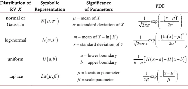
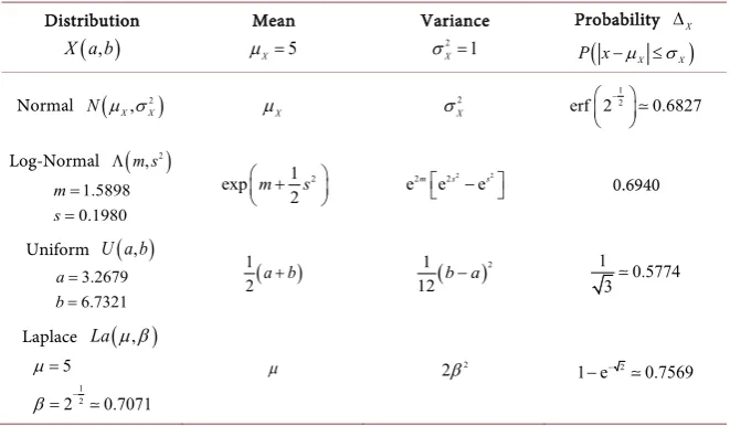
For comparison, Figure 1 shows plots of the PDF of a normal and log-normal distribution, as well as the PDFs of a uniform and Laplace distribution (which will be used in Section 3), all of the same mean

(

µX =5

)

and standard

devia-tion

(

σX =1

)

. The figure illustrates that the significance of the standard

devia-tion as a measure of statistical uncertainty (i.e. the width of the PDF) can vary markedly for different distributions, as summarized quantitatively in Table 2, which records the cumulative probability

( )

d

X X X X

X p x xX

µ σ µ σ

+ −

(8)

[image:8.595.263.489.66.290.2]

Figure 1. Graphical comparison of selected distributions of fixed mean

5

x

µ= = and fixed standard deviation _σ ₌ _x2 ₋_µ2₌₁_{: (a) Gaussian}

(red), (b) log-normal (black), (c) uniform (blue), (d) Laplace (green).

Table 2. Comparative significance of 1 standard deviation uncertainty. Distribution

( )

,

X a b

Mean 5 X µ =

Variance

2 ₁

X σ =

Probability ∆X

(

X X

)

P x−µ ≤σ

Normal

(

_, 2

)

X X

N µ σ µ_X 2

X

σ _{erf 2}_ −12_ _0.6827

 

Log-Normal _Λ

(

_{m s}_, 2

)

1.5898 0.1980 m s

= =

2

1 exp

2

m s

 ₊ 

 

 

2 2

em_es ₋es _

  0.6940

Uniform U a b

( )

,

3.2679 6.7321 a b = =

( )

1

2 a b+ ( )

2

1 12 b a−

1 _0.5774 3

Laplace La

(

µ β,

)

1 2

5

2 0.7071 µ

β −

=

= 

µ ₂_β2 _{1 e}₋ −2 _0.7569



Note that for variables N, U, and La the probability ∆X that a sample falls within ±1_{standard deviation of the mean is a constant dependent on the type}

of distribution, but independent of the parameters of the distribution. For the log-normal variable, however, ∆Λ has a complicated dependence on µΛ and

σ_Λ

(

)

(

)

( )

(

)

( )

2 2

2

1

ln ln ln

1 _erf 4

2 _2ln _4ln

µ σ µ σ µ

µ σ µ

Λ Λ Λ Λ Λ

Λ

Λ Λ Λ

   ₊ ₊ ₊ ₋ 

  _ _

  

∆ =

  ₊ ₋ 

 

 _ _

[image:8.595.209.540.376.569.2]

(9)

(

)

(

)

( )

(

)

( )

2 2 2 1

ln ln ln

4 erf

2ln 4ln

µ σ µ σ µ

µ σ µ

Λ Λ Λ Λ Λ

Λ Λ Λ

   ₋ ₊ ₊ ₋      _      −   ₊ ₋      (18)

where the error function is defined by

( )

2

0 2

erf e d

π

x _t

x _≡ − t

∫

. (19) The first column of Table 2 shows the values of the distribution parameters that lead to the fixed mean (µ =X 5) and variance (σ =X 1) specified in the first row. The second and third columns of the table provide the theoretical relations connecting the parameters of each distribution to the mean and variance of the associated RVs.

In the analyses and experiments of this paper, it will be adequate to neglect the skewness of Y and adopt MGF (16), which identifies Y as a normal RV. In that case, it follows that Z takes the form

eY eY YW

Z ₌ ₌ µ +σ ₍₂₀₎ in which W N≡

( )

0,1 is a standard normal RV. The justification of Equation (20) is that an arbitrary normal RV

N

(

µ σ

,

2

)

_{can be written in the form}_[21]

(

_, 2

)

N µ σ = +µ σW _{. (21)}

Equation (20) leads directly by integration to the expectation values of Z

(

)

22

2 2 1

e exp e d

2π 1 exp 2 Y Y w k k W

k

Y Y

Z k k w w

k k

µ σ _µ _σ

µ σ − ∞ + −∞ = = +   = _ + _  

∫

(22)

where the PDF of W is given in Table 1 by setting

µ =

0

and

σ =

1

in the PDF of

N

(

µ σ

,

2

)

_.

From Equation (22), the mean and variance of the log-normal RV are then

(

)

(

( )

)

2

2 2 2

1 exp

2

exp 2 exp 2 exp

Z Y Y

Z Y Y Y

µ µ σ

σ µ σ σ

 

= _ + _

 

= −

(23)

and the inverse relations, which will be needed later, can be shown to be

(

)

(

)

(

)

2 2 2

2 2 2 2

ln

Y Z Z Z

µ µ µ σ

σ µ σ µ

= +

= + (24)

Although the RV Y is distributed symmetrically about its mean, the distribu-tion of Z itself is skewed. From Equation (22) the third moment about the mean, to which skewness is proportional, can be shown to be

(

)

3 3 ₃ 2 ₂ 3 _e3 Y _e92 Y2 _e52 Y2 _e32 Y2

Z Z Z

Z₋_µ ₌ Z ₋ Z _µ ₊ _µ ₌ µ _ σ ₋ σ ₊ σ _

 

(10)

It is useful to note that Equation (20) provides an even more direct way than integration of the PDF at arriving at Equation (22) for the moments of Z since

e

k Yk

Z

=

_{takes the form of the MGF (16) of a normal RV, upon replacing} the dummy variable t with the moment order k.

The seminal findings of this section may be summarized as follows:

1) ArandomvariableZcomposedoftheproductof 2 ormorefactorRVsfor whichtheratioof standarddeviationtomeanis <1 isdistributed log-normally tothe extentthatthe skewness (andhigherordermoments) of ln

( )

Z canbe neglected.

2) Tofindtheparametersofthedistributionofalog-normalRVZ, onefirst transforms the data (e.g. sample or simulation) by yi =ln

( )

zi to obtain the

distributionoftheassociatednormalRVYwhichissymmetricaboutitsmean. In concluding this section, a point of comparison is in order regarding the CLT for the sum of independent RVs and relation (20) for the product of inde-pendent RVs. In brief, the CLT holds that the sum (e.g. mean) of a sufficiently large number N of identically distributed, independent RVs

(

,

)

, 1, ,

i X X

X µ σ i=  N converges to a normal RV irrespective of the distribu-tion of X, provided that the Xi have a well-defined mean and variance [22] [23]. In theory, the number N is infinitely large, but in practice it can be well be-low 10; see Ref [10], pp. 36-38. In contrast, the foregoing demonstration that a product of RVs is distributed approximately log-normally

(

)

( ) (

)

2

1 1

1

, ln ,

N N N

i i i i i i

i i

i

Z X µ σ µ σ µ

= =

=

 

= _{→ Λ } _



∑



∏

(26)

holds for any number of factors

N

≥

2

under the previously specified condi-tions. Moreover, the individual independent factors Xi

(

µ σi, i

)

need not have

identical distribution parameters, nor even all be the same type of variable X. The parameters of Λ shown in Equation (26) are from Equations (13), (14), (15) with neglect of the skewness parameter and terms of order

(

σ µ

i i

)

2 in the mean. This reduction has been found satisfactory in accounting for the Monte Carlo simulations and experimental results discussed in later sections.

2.2. Special Case: Product of Normal RVs

_X_i ₌_N_i

(

_{µ σ}

_i_, _i2

)

The log-normal distribution of a composite RV derived in the previous section is an approximate relation valid to the extent that certain conditions are fulfilled. In the special case where the factors Xi of the product (26) defining Z are normal RVs, an alternative expression for the PDF of Y =ln

( )

Z _{can be derived}

by means of the CF. This is an important case because the normal distribution satisfactorily describes measurements or estimates of many biomedical variables, physical variables, and variables relating to business management and finance, among others [24] [25] [26].

(11)

( )

1 1 j d e d

N N

it it iyt

Y j j X j j Y

j j

h t X x p x x p y y

= =

=

∏

=

∏∫

≡

_∫

₍₂₇₎

for the CF of Y, where the summation index has been changed from i to j so as not to be confounded with the unit imaginary i= −1_{. The inverse Fourier}

transform of Equation (27) then yields the PDF of Y

( ) ( )

( )

1

2π e d

2π e _j d d

iyt

Y Y

N

iyt it

j X j j

j

p y h t t

x p x x t

∞ − − −∞ ∞ − − −∞ = =   = _ _  

∫

∏

∫

(28)

in which the second equality of Equation (27) was substituted for h tY

( )

in the

first line of Equation (28). The PDF of Z is calculable from the PDF of Y by the following transformation (see Appendix 1):

( )

1

(

_ln

( )

)

Z Y

p z

₌

z p

−

z

_{. (29)} Substitution of relation (21) for each normal factor Xj into (27) leads to

( )

1

(

)

2₂

2

1 2π j j e d

N _it

x

Y j j

j

h t − ∞_{µ σ} µ σ x − x

− =

=

∏

_∫

+ _{, (30)}

which can be re-expressed in the form

( )

( ) 1

(

)

1 _ln

2 2

1 2π e exp ln 1 2 d

j j

N _it

Y j

j

h t µ _α− it α x x x

∞ −

− =

=

∏

_∫

+ − ₍₃₁₎

where

j j j

α =σ µ _{. (32)}

Equation (31) is an exact expression for the CF of Y, but, to the author’s knowledge, cannot be integrated in closed form. However, for αj <1, expan-sion of the logarithm in a Taylor series to order 2

j

α

results in the closed form expression

( )

(

)

2 2 2

2 1 1 exp 1 2 1 it

j j j

N Y

j _j

t i t

h t

i t

µ α α

α =  ₋ ₊     _ _   =  +     

∏

. (33)

Substitution of CF (33) into Equations (28) and (29) provides a more accurate PDF of Y and Z than the PDF of log-normal (26).

If 2 ₁ j

α < for each factor in Equation (27), then one can approximate

( )

Y

h t in Equation (33) by

( )

2 2

1 1 exp 2 N it

Y j j

j

h t µ α t

=

₋ 

 

 

∏

 (34) which, substituted into the integral in Equation (28), leads to the Gaussian dis-tribution

(

₂

)

( ) (

)

2

1 1

1

ln N _i _i, _i N ln _i ,N _i _i

i i

i

Y N µ σ N µ σ µ

= =

=

   

= _ _→ _ _

 

(12)

for Y and the log-normal distribution (26) for Z.

As an example to illustrate the stages of the analysis, consider the composite RV

(

)

( )

(

)

(

( )

)

(

( )

)

(

( )

)

4

1

2 2 2 2

1 2 3 4

,

1.0, 0.2 4.0, 0.5 6.0, 1.0 10.0, 1.5 i i i

i

Z X

N N N N

µ σ =

=

∏

(36)

and associated log-product Y =ln

( )

Z _{. In}_{Figure 2}_{are plotted the real part}

( )

Re F (red), imaginary part Im

( )

F (blue), and magnitude F (dashed black) of the Fourier transform F t

( )

=h tY

( )

given by Equation (33) as a

func-tion of t. Although t serves in the MGF as a dummy variable for computation of statistical moments by differentiation, in the CF t is equivalent to a spatial or temporal frequency [27] [28]. F and Re

( )

F are seen to be symmetric, and

( )

Im F antisymmetric, about t = 0, extending over a range ∆ ≈t 20_{from −10}

to +10. Figure 3 shows plots of p yY

( )

, Equation (28), as calculated by (1)

nu-merical integration of the Fourier transform of the exact CF (31) (solid red), (2) the analytical approximation (33) to the CF (dashed blue), and (3) the PDF of the normal RV (35) (solid green). Profiles (1) and (2) are seen to be nearly indis-tinguishable, and both are well approximated by the Gaussian profile (3). Figure 4 shows plots of p zZ

( )

as calculated by (1) numerical integration of the

transformation (29) of the exact PDF of Y (solid red), and (2) the PDF of the approximate log-normal RV (26) (dashed blue). The exact and log-normal PDFs of Z closely match, apart from a slight forward shift of the peak of the log-normal profile.

2.3. Special Case: Product of Log-Normal RVs

X_i _{= Λ}_i

(

m s_i_, _i2

)

The ubiquity of the normal distribution is primarily a consequence of the CLT, which is a limiting theorem for the sum of a large (in theory, infinite) number of random variables. Moreover, the distributed variable can take—or, as a matter of practicality, be thought to take—both positive and negative values, since the Gaussian PDF is normalized to unity only when integrated over the entire real axis. The log-normal distribution also occurs widely, particularly in reference to activities that involve counting, measuring, or observing the attributes of real physical things. Such activities underlie many kinds of problems for which crowdsourced solutions can be sought. The distributed variable then takes on only non-negative real values and is expected to be intrinsically skewed, since its least value cannot be below zero, whereas its upper limit is open.

Consider, therefore, a composite variable Z comprised of log-normal factors

(

2

)

1

, N

i i i i

Z m s

=

∏

Λ ₍₃₇₎

with PDF of the form (see [21], pp. 131-134)

(

)

1

(

( )

)

2 ₂

)

, exp ln 2

2π

Z

p z m s z m s

sz

(13)

[image:13.595.260.491.69.224.2]

Figure 2. Fourier transform F t

( )

of the characteristic function of

( )

ln

Y= Z _{, Equation (33), where} 4

(

2

)

1

,

i i i i

Z N µ σ

=

∏

is defined by para-meters µi=

{

1.0,4.0,6.0,10.0

}

and σi=

{

0.2,0.5,1.0,1.5

}

: (a) real part

[image:13.595.262.489.313.450.2]

(solid red), (b) imaginary part (solid blue), (c) magnitude (dashed black).

Figure 3. PDF of Y=lnZ_{defined in} Figure 2, as calculated from the Fourier transform of the exact CF Equation (31) (solid red), the Fourier transform of the analytical approximation Equation (33) (dashed blue), and the Gaussian Equation (35) (solid green).

[image:13.595.262.487.521.679.2]

(14)

It then readily follows from the inverse of Equation (29) (see Appendix 1) that the PDF of the variable Y =ln

( )

Z has the form

(

_,

)

1 _exp

(

)

2 ₂ 2

)

2π

Y

p y m s y m s

s

= − − ₍₃₉₎

which shows that Y is a Gaussian RV of mean m and variance _s2_,_i_._e_.

( )

_,

2

Y N m s

=

_.

Thus, taking the log of Equation (37) leads to the chain of relations

( )

(

2

)

(

2

)

2

1 1 1 1

ln N ln i i, i N i i, i N i, N i

i i i i

Y Z m s N m s N m s

= = = =

 

= = Λ = _{= } _

 

∑

∑ ∑

(40)

from which it follows that Z, itself, is a log-normal RV

( )

_,

2

Z

= Λ

m s

₍₄₁₎ with 1 2 2 1 N i i N i i m m s s = = = =

∑

(42)

Stated formally: Theproductoflog-normalRVsisalog-normalRVwith pa-rametersgiven by Equation (42). Note that the preceding result, Equation (41), is exact; no approximations regarding either the number of factor RVs or the relative magnitudes of parameters mi and si have been made.

From Equation (23) the mean and variance of Z, defined by Equation (37), is then

2

1 1

2 2 2

1 1 1

1 exp

2

exp 2 exp 2 exp

N N

Z i i

i i

N N N

Z i i i

i i i

m s

m s s

µ σ = = = = =   = _ + _           = _ __ _ _− _ __      

∑

(43)

3. Monte-Carlo Simulations of a Composite Random Variable

In this section the distribution of responses to the kind of archetypical problem posed at the end of Section 1.1 is examined numerically by means of Monte-Carlo simulations (MCS) employing four basic types of two-parameter RVs Xi

(

µ σi, i

)

: 1) normal, 2) uniform, 3) Laplace, and 4) log-normal. The

means µi and standard deviations σi of the factor RVs are respectively those of the arguments of the four RVs in Equation (36):

(

) (

)

(

) (

)

(

) (

)

(

) (

)

1 1 2 2 3 3 4 4 , 1.0,0.2 , 4.0,0.5 , 6.0,1.0 , 10.0,1.5 µ σ µ σ µ σ µ σ = = = = (44)

(15)

represent the numerical density of objects in a receptacle, and the variables 2, ,3 4

X X X to characterize the 3-dimensional receptacle geometry. The physical quantity for which an estimate is sought is then represented by the variable

1 2 3 4

Z X X X X= _{. If}_Z_{is satisfactorily described by a log-normal RV, then}

(

1 2 3 4

)

ln

Y = X X X X _{should be well-approximated by a Gaussian RV.}

Each of the four simulations of the composite variable Z reported in the sub-sections to follow comprises independent samples from a random number generator (RNG) corresponding to one of the four basis RVs listed above. The simulated variates

{ }

x

i j,

(

i=1, 2,3, 4;j=1, , n

)

are partitioned into uniform bins of width

∆ =

x

0.1

; the resulting variates

{ }

y

j ,

{ }

z

j are partitioned into uniform bins of width

∆ =

y

0.1

, ∆ =z 10.0_(if X N U La= , , ) or 15.0 (if X = Λ_{). To get a sense of scale, note that the product of the four} means in Equation (44) is 240 and that ln 240

(

)

≈5.48. It is to be expected, therefore, that, neglecting skewness, the histogram of Z should be centered at a point near 240, whereas the symmetric histogram of Y should be centered at close to 5.48, which lies between the centers of histograms X2 and X3.

Superposed on each of the generated histograms in the figures to follow will be the relevant theoretical PDF (solid red): 1) PDF of the corresponding RNG for the basis variables

{ }

Xi , 2) log-normal PDF (26) (if X N La U= , , ) or (41)

(if X = Λ_{) for}Z_{, and 3) normal PDF (35) (if} X N La U= , , ) or (40) (if X = Λ₎ for Y. The analysis of Section 2.1 leads to an important prediction concerning the four Monte Carlo simulations:

• _Each_simulation_,_although_generated_with_a_different_type_of_basis_variable_X_,

shouldleadwithinstatisticaluncertaintiesto identicalhistograms forZ and Y.

The preceding prediction follows from the fact that the means and variances of Z and Y depend only on the means and variances (44) of the basis variables

i

X , and not on the type of RV symbolized by X. From the ungrouped variates of each MCS

1, 2, 3, 4,

j j j j j

z =x x x x ₍₄₅₎

(

1, 2, 3, 4,

)

ln

j j j j j

y = x x x x _{, (46)}

one can calculate the sample mean and sample variance of Z by two different approaches, both employing relations deduced from the method of maximum likelihood (ML) [29]. The first approach is to calculate the sample mean

( )

mZ

and sample variance

( )

2 Z

s

directly from the set of variates (45)

SAMPLE: Z

(

)

1

2 2

1

1 n

Z j

j n

Z j Z

j

m z

n

s z m

n

=

= −

∑

(47)

The second approach is to calculate the sample mean

( )

mY and sample

(16)

SAMPLE: Y

(

)

1 2 2 1 1 1 n Y j j n

Y j Y

j

m y

n

s y m

n = = = = −

∑

(48)

and use relations (48) to deduce the sample mean

(

MZ

)

and sample variance

( )

2 Z

S as follows from Equation (23)

SAMPLE: Z(Y)

(

)

(

( )

)

2

2 2 2

1 exp

2

exp 2 exp 2 exp

Z Y Y

Z Y Y Y

M m s

S m s s

 

= _ + _

 

= −

(49)

Agreement of statistics (47) and (49) would be indicative that the variates of Z

were distributed log-normally.

Comparison of sample statistics with theory for each of the simulations to follow are summarized in Table 3.

3.1. Normal Basis

X

=

N

The normal distribution is defined by its mean and variance (see Table 1). The basis variables of the simulation are therefore Ni

(

µ σ

i, i2

)

, i=1,2,3,4, as shown in Equation (36) with parameters as defined in list (44). For purposes of comparing histogram shapes, it is noted that the skewness and kurtosis of a normally distributed RV are respectively

( )

₍

₎

3

0 N

X X X

Sk ≡ X −µ σ = (50)

( )

₍

₎

4

3 N

X X X

[image:16.595.211.540.518.732.2]

K ≡ X−µ σ = . (51) Skewness (50) is a measure of symmetry of the PDF with respect to the mean. Kurtosis (51) is a measure of the shape of the tails of the PDF. A distribution

Table 3. Statistics of Monte Carlo simulations of Z X X X X= 1 2 3 4.

Basis Parameters

(

,

) (

1,2,3,4

)

i i i

X µ σ i=

(

µ σi, i

) (

=1,0.2 , 4,0.5 , 6,1.0 , 10,1.5

) (

)

Sample (n = 1,000,000)

Theory

(

_, 2

)

Y Y

Z= Λ µ σ

Basis Variables Xi Sample Z Sample Y Sample Z(Y) Y Z Normal Z _79.54240.01

Z m s = = 5.43 0.34 Y Y m s = = 240.48 83.91 Z Z M S = = 5.48 0.33 Y Y µ σ = = 253.05 84.58 Z Z Μ = Σ =

Uniform Z _79.53240.02 Z m s = = 5.43 0.33 Y Y m s = = 240.23 82.11 Z Z M S = = — —

Laplace Z _79.48240.01 Z m s = = 5.42 0.38 Y Y m s = = 243.01 96.58 Z Z M S = = — —

(17)

with “fat tails” (leptokurtic) has a higher probability than normal of extreme events, in contrast to a distribution with “thin tails” (platykurtic) for which the probability of extreme events is lower than normal.

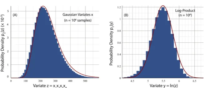
Figure 5 shows a panoramic plot of the histograms of X1 (green), X2, X3, 4

X (gray), and Y =ln

(

X X X X1 2 3 4

)

(blue), where Z X X X X= 1 2 3 4. As ex-pected, all the histograms in the figure appear to be Gaussian, and the histogram of Y lies between the histograms of X2 and X3.

Panels A and B of Figure 6 respectively show in greater detail the histograms of Z and Y, bordered by the profiles of the corresponding log-normal and nor-mal PDFs. In panel A, the right tail of the histogram is marginally less skewed than predicted by the log-normal model. In panel B, the left tail of the histogram is marginally more skewed than the symmetric profile of the Gaussian PDF. Nevertheless, in both panels, the theoretical profiles satisfactorily match the peak and overall shape of the histograms.

3.2. Uniform Basis

X

=

U

A uniform RV X

(

µ σ,

)

=U a b

( )

, is symbolized by its upper and lower boun-daries

(

b a>

)

. From Table 2 it follows that the mean and standard deviation of

X are related to the boundary parameters by

3 3

a b

µ σ

= −

= + (52)

The basis RVs Xi

(

µ σi, i

)

,i=1, 2,3, 4 of the simulation, which have the same

[image:17.595.254.492.449.628.2]

means and variances as the basis RVs of Section 3.1, are then respectively

Figure 5. Monte-Carlo simulated histograms of normal variables

(

_,

)

(

_, 2

)

i i i i i i

X µ σ =N µ σ _{with means}µ_i_{and standard deviations}σ_i_{listed in} (44), and 4

1

ln i i

Y X

=

 

= _

∏

_ (blue). X1 (green) represents number density; X2, 3

X , X4 (gray) represent geometric dimensions. The sample size is n=106.

(18)

[image:18.595.211.538.63.205.2]

Figure 6. Panel A: Histogram of Gaussian product Z of Figure 5 enveloped by PDF of log-normal variable (26) with values (44). Panel B: Histogram of Y=ln

( )

Z _of_{Figure 5}

enveloped by PDF of Gaussian variable (35).

(

)

(

)

(

)

(

)

1 1

2 2

3 3

4 4

0.6536,1.3464 3.1340,4.8660 4.2679,7.7321 7.4019,12.5981

X U

= = = =

(53)

The skewness and kurtosis of a uniformly distributed RV are ( )U ₀

X

Sk = (54) ( )U _{9 5 1.8}

X

K = = _{. (55)}

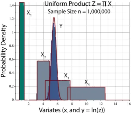
Figure 7 shows a panoramic plot of the histograms Xi, which have tails that drop vertically in comparison to the Gaussian histograms of Figure 5. Equation (55) establishes that a uniform RV is platykurtic, as is apparent from Figure 1. Nevertheless, the histogram of Y=ln

(

X X X X1 2 3 4

)

is again well represented by

a Gaussian PDF, which indicates that Z X X X X= 1 2 3 4 should be reasonably well described by a log-normal RV, as shown in greater detail in Figure 8.

3.3. Laplace Basis

X

=

La

A Laplace RV X

(

µ σ,

)

=La

(

µ β,

)

is symbolized by a location parameter

µ

corresponding to the mean of X and a scale parameter

β

_{related to the} stan-dard deviation of X by

1 2

2

β= − σ ₍₅₆₎

(see Table 2). The four basis variables of the simulation, which have the same means and variances as the basis RVs of Section 3.1, are then respectively

(

)

(

)

(

)

(

)

1 1

2 2

3 3

4 4

1.0,0.1414 4.0,0.3536 6.0,0.7071 10.0,1.0607

X La

= = = =

(57)

(19)

[image:19.595.265.480.74.258.2]

Figure 7. Monte-Carlo simulated histograms of uniform variables Xi

(

µ σi, i

)

=U a bi

(

i, i

)

with means µi and standard deviations σi listed in (44), and

4

1

ln _i

i

Y X

=

 

=  



∏

. Histo-grams Xi are enveloped by their associated uniform PDFs (red). Histogram Y is

[image:19.595.213.535.363.513.2]

enve-loped by the Gaussian PDF of Figure 5. Sample size, symbolic notation, and color coding are the same as in Figure 5.

Figure 8. Panel A: Histogram of uniform product Z of Figure 7 enveloped by PDF of log-normal variable (26) with values (44). Panel B: Histogram of Y=ln

( )

Z of Figure 7

enveloped by PDF of Gaussian variable (35). ( )La ₀ X

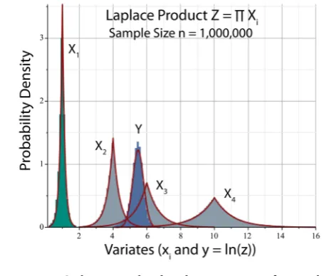
Sk = ₍₅₈₎ ( )La ₆

X

K = . (59) Figure 9 shows a panoramic plot of the histograms Xi, which have sharp cusps and fat tails in comparison to the Gaussian histograms of Figure 5. Equa-tion (59) establishes quantitatively that a Laplace RV is leptokurtic, as is appar-ent from Figure 1. Nevertheless, the histogram of Y =ln

(

X X X X1 2 3 4

)

is again

(20)

[image:20.595.254.482.74.268.2]

Figure 9. Monte-Carlo simulated histograms of Laplace variables

(

,

)

(

,

)

i i i i i i

X µ σ =La µ β _{with means}µ_i_{and standard deviations}σ_i_{listed in (44), and}

4

1

ln i i

Y X

=

 

= _

∏

_. Histograms Xi are enveloped by their associated uniform PDFs (red).

Histogram Y is enveloped by the Gaussian PDF of Figure 5. Sample size, symbolic nota-tion, and color coding are the same as in Figure 5.

Figure 10. Panel A: Histogram of Laplace product Z of Figure 9 enveloped by PDF of log-normal variable (26) with values (44). Panel B: Histogram of Y=ln

( )

Z of Figure 9

enveloped by PDF of Gaussian variable (35).

3.4. Log-Normal Basis

X

= Λ

A log-normal RV

_X

(

_{µ σ = Λ}

_,

)

( )

_{m s}

_,

2 _{is symbolized by the mean and variance} of the normal variable _{Y N m s}₌

(

_, 2

)

₌_ln

( )

_X _{. From Equation (24), re-expressed}

below for convenience,

(

)

(

)

(

)

2 2 2

2 2 2 2

ln

m

s

µ µ σ

µ σ µ

= +

= + (60)

[image:20.595.212.537.363.516.2]

(21)

(

)

(

)

(

)

(

)

1 1

2 2

3 3

4 4

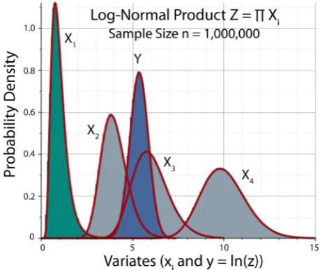
0.0196,0.1980 1.3785,0.1245 1.7781,0.1655 2.2915,0.1492

X X X X

= Λ − = Λ = Λ = Λ

(61)

The skewness and kurtosis of a log-normal RV ( )

(

_exp

( )

2 _{2 exp}

)

( )

2 ₁

X

SkΛ ₌ s ₊ s ₋ ₍₆₂₎

( ) _{exp 4}

( )

2 _{2exp 3}

( )

2 _{3exp 2}

( )

2 ₃ X

K Λ ₌ s ₊ s ₊ s ₋

(63) are not constants, but depend on the scale parameter s. Skewness (62) is greater than 0 for all values of s>0_{; kurtosis (63) is greater than 3 for all values of}

0

[image:21.595.207.537.72.207.2] [image:21.595.258.488.438.632.2]

s> _.

Figure 11 shows a panoramic plot of the log-normal histograms Xi, which skew to the right in comparison to the symmetric shapes of the Gaussian basis histograms of Figure 5. The histograms of Y =ln

(

X X X X1 2 3 4

)

and

1 2 3 4

Z X X X X= _{are seen to be precisely normal and log-normal, respectively, as}

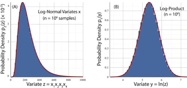
predicted in Section 2.3 and shown in detail in Figure 12.

3.5. Commentary

The set of variates (45) comprise the response of a crowd to a problem for which the sought-for solution is a composite random variable Z. The information, or so-called “wisdom of the crowd” [1], lies in the distribution of Z from which the full population statistics can be determined. In comparing the MCS histograms

Figure 11. Monte-Carlo simulated histograms of log-normal variables

(

_,

)

(

_, 2

)

i i i i i i

X µ σ = Λ m s with means µi and standard deviations σi listed in (44),

and 4

1

ln i i

Y X

=

 

= _

∏

_. Histograms Xi are enveloped by their associated log-normal

(22)

[image:22.595.212.535.74.226.2]

Figure 12. Panel A: Histogram of log-normal product Z of Figure 11 enveloped by PDF of log-normal variable (41). Panel B: Histogram of Y=ln

( )

Z of Figure 11 enveloped by PDF of Gaussian variable (40).

of Y and Z to the profiles of their respective PDFs, one should bear in mind that in general there is no underlying fundamental theory of crowd response. The log-normal model is not a fundamental theory such as one encounters in physics, and therefore the MCS histograms in Section 3 were not subjected to a chi-square goodness-of-fit test, as is often done in physics to compare experi-ment and theory.

The validity of the analytical model developed in this paper lies in how well it enables the analyst to predict an unknown quantity represented by the sampled variable Z, and not necessarily in how closely the complete distribution of the sample (i.e. histogram of Z) is matched by a log-normal distribution. However, if there is reason to believe that the basis variables Xi comprising the composite variable Z are distributed log-normally, then Z itself should be rigorously log-normal, and a goodness-of-fit test may then be appropriate. This point will be illuminated further in Section 4, which reports a crowdsourcing experiment and MCS to estimate the number of identical objects in a receptacle.

The preceding comments notwithstanding, Figures 5-12 illustrate how well the predicted log-normal distribution fits the histograms of Z generated by basis variables of widely differing distribution shapes, as distinguished by their skew-ness and kurtosis. Simulations using normal or log-normal basis variables yielded the visually closest matches to the log-normal model. In the case of a log-normal basis, theory predicted, and MCS sustained, an exact log-normal dis-tribution of Z.

4. Test of Crowdsourced Estimation

(23)

experiments were performed entailing crowdsourced estimates of 1) the weight of a tangible local object, and 2) the quantity of a remotely viewed object. (See Ref. [10] for a popular account.) Experiments of these kinds were conducted by the author in various physics classes during the past two decades, but no single sample was large enough to permit reliable inference of the statistical distribu-tion. Pooling of results from different sample populations was not feasible since the conditions of the experiments were not all identical.

4.1. The Coin-Estimation Experiment

The experiment analyzed in detail here is of the second kind. Viewers of The One Show were shown on their televisions a transparent tumbler filled with opaque £1 coins. The tumbler rested on a table adjacent to two ordinary cylin-drical glasses of water to provide clues to scale. No explicit dimensions of any objects were given. The challenge posed to viewers (i.e. the crowd) was to esti-mate the number of coins in the vessel.

The experimental estimates ( )exp k

z , k=1, , n0, were transmitted to the show by email, and the author subsequently received the full set of n0=1706 ano-nymous responses, which ranged from a low of 42 to a high of 43,200.1_The mean and median of the estimates were respectively _Z(exp) ₌₉₈₂_, _Z_(exp) ₌₆₉₅_. The true count was Nc=1111. If the mean is taken as the measure of crowd

response—a standard statistical practice—the fractional error of the crowd was ( )exp

(

( )exp

)

_11.6%

c c c

N Z N N

∆ = − = − _{. (64)}

Although result (64) is not bad, it calls into question—at least to the au-thor—how Galton’s crowd of just 800 members (less than half the BBC sample size) could guess the weight of an ox to within a fractional error of less than 0.1%. One explanation might be that the participants at the fair comprised a crowd of experts familiar with livestock. The respondents to The One Show apparently had no special expertise in the estimation of quantity.

Figure 13 shows a scatter diagram of the estimates as a function of sample number, i.e. the order in which the estimates were received. Estimates in the ap-proximate range between 0 and 1000 form a dense band; estimates from about 2000 to 10,000 resemble a foam of points the density of which falls off with in-creasing ordinate. The blue histogram labeled “Experiment” in Figure 14 shows the distribution of estimates partitioned over K = 24 bins of equal width ranging from 0 to 4000. Points that extended beyond 4000 are not shown, since the main body of the histogram would then be severely compressed. Superposed on the histogram of experimental results is the profile (dashed blue) of the correspond-ing log-normal PDF with sample parameters obtained by application of the me-thod of maximum likelihood (ML) to a Gaussian _Y( )exp _[30]_,

1_{Actually, the maximum value submitted was 25 million, which was about 15% of the entire BBC}

(24)

[image:24.595.267.483.67.264.2]

[image:24.595.264.485.321.511.2]

Figure 13. Estimates, in order of receipt, of the number of £1 coins in a tumbler displayed on the BBC One Show in 2007. The true count was 1111 coins; the sample size was 1706. Statistics of the experiment are given in Table 4.

Figure 14. Comparison of the histogram (blue) of 1706 crowdsourced estimates with the histogram (gray) of 106_{Monte Carlo simulated responses employing}

log-normal basis variables for coin density and tumbler geometry. The crowd-sourced mean estimate was 982; the MCS mean was 1057; the true count was 1111. Relevant statistics are given in Table 4. Enveloping the histograms are the profiles of the log-normal PDFs for the sample (dashed blue) and simulation (solid red).

( )

0

exp 0

1 0

1 n _6.565

k k

m y

n =

=

∑

= ₍₆₅₎

( )

(

)

0 _exp 2

0 0

1 0

1 n _0.719

k k

s y m

n =

=

∑

− = ₍₆₆₎

where the variates ( )exp k

y are defined by ( )exp _ln

( )

( )exp

k k

(25)

Parameters m0 and s0 in Equation (65) are respectively the mean and standard deviation of _Y( )exp _{. The gray histogram with red border in}_{Figure 14} will be discussed in Section 4.2.

Despite the caution about goodness-of-fit tests in Section 3.5, it is noteworthy that the fit of the log-normal PDF with parameters (65) to the histogram of ex-perimental estimates actually does exceed the 5% acceptance threshold of a chi-square test for

ν

=21_{degrees of freedom:} 2

21 6.4%

χ = _{. The number}ν_of

degrees of freedom is given by

1 K

p

ν = − −

(68) where K = 24 is the number of distribution categories (bins), p = 2 is the number of parameters

(

m s0, 0

)

determined from the data, and the numeral 1 refers to

the fact that the histogram is normalized to unit area, in which case knowledge of the values of K−1 bins determines the value of the remaining bin.

4.2. Monte Carlo Simulation of the Coin Estimation Experiment

Passing a goodness-of-fit test does not necessarily prove that a hypothesized theory is correct. Rather, it signifies that the theory should not be rejected on the basis of the tested data. The statistical significance of the experiment described in Section 4.1 is that the distribution of estimates of the number of coins (a composite RV) is consistent with a log-normal distribution for the given sample. Nevertheless, the implication of this result is of far-reaching practical impor-tance:

Ifitisindeedthecasethattheestimatesfromacrowdofgivensizeare distri-butedlog-normally, thenoneshouldbeabletosimulatetheestimatesofamuch largercrowdbyconstructingtheappropriatebasisvariablesthatformthefactors ofthesought-forcompositevariable.

In other words, the analyst may be able to avoid sampling an impractically large crowd, yet still obtain reliable statistical information by a Monte Carlo si-mulation (MCS). In this section the responses from a hypothetical crowd of 1 million were simulated by applying the underlying reasoning and mathematical procedure described in Section 2.