Online Full Text



Abstract—To select the best alternative of solution for a

problem considering the decision-maker knowledge, preferences and purposes, we developed a new multicriteria decision-making procedure, the PROV Exponential Decision Method, which uses the concepts of preference, indifference and nefarious thresholds. Its presentation is the main focus of this article. Numerical examples are presented to illustrate the proposed approaches to attain comprehensible results and to discover the most adequate solution or set of solutions for a problem or to select the best option to reach a defined goal.

Index Terms—Exponential normalization, multicriteria

decision-making, projects assessment, projects selection and prioritization.

I. INTRODUCTION

ULTICRITERIA decision methods are applied to find the most appropriate solution for a specific problem or to attain a certain goal, providing an ordering of the options, from the best to the least performing option, having per reference their different criteria attributes or features and their relative weights. There are numerous multicriteria decision methods, and many of them try to establish procedures, based on preference or concordance thresholds, to avoid linear drawbacks, since the criteria attributes may not have a linear progression for the decision-maker, and as far as we know, there is any complete multicriteria decision method using the exponential normalization to express the decision maker knowledge, preferences and purposes. On this article we present a new procedure, that we called the PROV Exponential Decision Method (decision-maker Preferences Ranking and Options Value based on the linear and on the exponential normalization), to overcame the limitations of linear approaches and to avoid the uncertainty associated with the assignment of preference or concordance thresholds [8]. Among the most known multicriteria decision methods addressing the decision-maker preferences are the AHP (Analytic Hierarchy Process) [1], [3], [7] the ELECTRE (Élimination et Choice Traduisant la Réalité) [2], [4] and the PROMETHEE

Manuscript received March 06, 2012; revised April 20, 2012.

This work was supported by the QREN – Operational Programme for Competitiveness Factors, the European Union – European Regional Development Fund and National Funds – Portuguese Foundation for Science and Technology, under Project FCOMP-01-0124-FEDER-011377 and Project Pest-OE/EME/UI0252/2011.

António Rocha is a PhD student at the Department of Production and Systems of the University of Minho, Portugal (e-mail: [email protected]).

Anabela Tereso is an Assistant Professor at the Department of Production and Systems of the University of Minho, Portugal (e-mail: [email protected]).

(Preference ranking organization method for enrichment evaluations) [5]. The ELECTRE and PROMETHEE are outranking methods which use reference threshold to encompass the limitations of the linear normalization. AHP uses a nine-points importance scale to rank the options and their criteria through paired-wise comparisons. The PROV Exponential Decision Method uses the concepts of preference, indifference and nefarious thresholds but they are used on a graphical representation where we can observe the relative position of every option on two lines, the linear and the exponential line to determine the values best representing the decision-maker thoughts and intentions. The presentation of this method is provided in four sections where we define its scope and purpose, present its application procedure, make some further considerations about nefarious values and finally present the conclusion and lines for further research.

II. SCOPE AND PURPOSE

The PROV Exponential Decision Method was developed to express the stakeholders knowledge, objectives and preferences to attain comprehensible results and to discover the most adequate solution for a problem or to accomplish a certain goal and the ordering and relative value of the alternative solutions. Through the modelation of the stakeholders thoughts and purposes this method allow us to develop an informed evaluation having in mind all the options which are visually shown on a graphical representation. This graphical representation presents the options relative position on two lines, one expressing a linear growth which means that increments of the same size have equal importance, and another line expressing the real value attributed by the decision-maker having into account that as some milestones are attained, the importance attributed to greater values may decrease, since some value of satisfaction has been attained. It also lets the decision maker express the interval of values at which he considers the options indifferent among each other. He can also express that the options in a determined interval of values have a closer importance and as they get away from this interval the value of those options decrease intensively. The decision-maker can also express the decrease of preference if, at a determined level the continuous growth, it becomes nefarious for the problem under analysis.

Whenever we are on the presence of more than one criterion and more than two options of choice the PROV Exponential Decision Method can be applied. It can be particularly important on investment decisions, on product portfolio assessment and on the evaluation of intangible assets and intellectual capital. But most of all, it is a useful method for policy appraisal and public funding, concerning social interventions, the environment and quality, and health

Prov Exponential Decision Method

António Rocha, Anabela Tereso, and Paula Ferreira

and safety issues. Its main relevance is also expressed for products and equipments acquisition and implementation.

III. APPLICATION PROCEDURE

The application of the PROV Exponential method can be understood by following the subsequent steps:

1st Establish the overall objective to be achieved;

2nd Enounce the main requisites that a solution for the problem will have to accomplish;

3rd Identify reasonably practicable alternatives (options) of solution (it is advisable to look for similar problems to find existent solutions);

4th Enounce all the options relevant criteria to be taken into account during the analysis;

5th Identify the attributes for each option and establish a matrix with these attributes; if all the criteria or part of them are qualitative, establish Likert scales to make them quantifiable (every criterion may have their own independent reference scale; a posteriori, they will be normalized in a scale between 0 to 1);

TABLE I- ATTRIBUTES OF EVERY OPTION

Options

Criteria o1 o2 o3 o4 om

c1 x11 x21 x31 x41 xm1

c2 x12 x22 x32 x42 xm2

c3 x13 x23 x33 x43 xm3

cn x1n x2n x3n x4n xmn

6th Analyze the attributes of the options to verify if the lowest performance of some option, in fundamentally important criteria, makes them unacceptable (this should be done if we have crucial criteria demanding minimum standards to avoid possible compensation by other criteria; the options below the minimum standards shouldn’t be considered);

7th Determine or assign weights to the criteria. The weights can be assigned directly by the decision-maker and the problem stakeholders or they can be attained using criteria weighting methods. Nevertheless the stakeholders should always review the results of the application of weighting methods to assure that the assigned weights really reflect their knowledge and objectives;

8th Determine the criteria to be maximized (the higher values are the best condition) and to be minimized (the lower values are the best condition) and apply the exponential normalization procedure to the attributes of table 1, according to the following formula (1), where x is obtained by a linear normalization procedure and a corresponds to an independent factor expressing the decision-maker knowledge, preferences and purposes. Establish a graph containing two lines (the linear normalization line and the exponential normalization line).

(1)

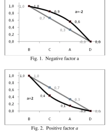
A negative factor a results in a concave exponential growth (Fig. 1). A positive factor a results in a convex one (Fig. 2).

Fig. 1. Negative factor a

Fig. 2. Positive factor a

A negative factor a brings closer the best options and detaches them from the less performing ones. By making factor a more negative those differences become even more significant. A positive factor a brings the decision-maker closer to the best option detaching it from the others by increasing the proximity between the less performing ones. By making factor a more positive the proximity between the less performing options is augmented. Therefore, it is possible to adequate the values according to the decision-maker perceptions by changing factor a [6]; we can also have more than one factor a.

9th Analyze the lines progression and change factor a to reflect the decision-maker knowledge, preferences and objectives. The decision-maker should take into account the options criteria linear progression and the reference scale between 0 and 1. This reference scale should be taken as a measure of importance or concordance to translate the decision-maker thoughts and intentions. The options are more important as they approach 1 and decrease their importance as they decrease till 0. The graph offers a good visual representation of the options relative value and we can make judgments having in mind all the options under evaluation. In this way, we are not only making paired-wise comparisons; we are also performing an integrated assessment of all the options since we can observe the relative position of all of them in the linear and on the exponential line.

Exponential normalization

Higher value is the best condition(maximization)

Expij=

ea×x−1

ea−1

,where x= x

ij−Min xij

Max xij − Min xij

Lower value is the best condition(minimization)

Expij=

ea×x−1

ea−₁ ,where x=

Max xij−xij

Max xij− Min xij

x−corresponds to a linear normalization procedure

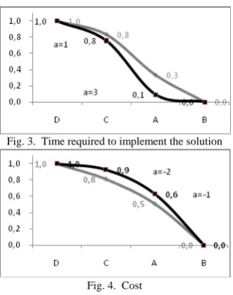
Fig. 3. Time required to implement the solution

Fig. 4. Cost

On Fig. 3 and 4 we can observe how factor a supports the modeling of the decision-maker thoughts and intentions by assigning more than one factor a to bring the options closer or detached from each other. In Fig. 3 we have two factors a (1 and 3). The first expresses a decrease of value stronger than a linear evaluation would suggest, but as the options get lower performances the detachment from the linear normalization line is even huger. This happens because we have a factor a with a value of 3 expressing a significant decrease of the value of option A, bringing it closer to the value of option B, which has the longest implementation time. In Fig. 4 we can notice that the decision-maker doesn’t make a significant distinction between the cost of the first two options, since we have a negative factor a which brings closer the best options and detaches them from the less performing ones. As the cost increases, the decision-maker changes the negative factor a from -2 to -1 meaning that he still considers the option value a bit greater than the one assigned by a linear value line, detaching it from the lowest performing option.

We can also graphically express indifference and nefarious threshold (the nefarious threshold will be analyzed later). The indifference threshold refers to a value over which the decision-maker doesn’t make any distinction between the options criteria and its establishment is important to avoid conditioning the options final result. This threshold can be graphically modeled by assigning a positive or negative factor a till a level at which the options became indifferent (with the same value) among themselves. If all options have exactly the same importance, we don’t need to model the options graphically, and we should assign to all of them their maximum criteria attribute.

Remark concerning steps 8th and 9th: The exponential normalization allow us to attain the exact internal difference between the options by establishing a reference scale between 0 and 1. The 0 corresponds to the lowest value and the 1 to the highest value, but by doing this comparison, the options inherent value is altered, for example: three students (A, B and C) have the following classifications: A(15), B(17) and C(18). If we just consider the exact internal difference between the students classification on a 0 to 1 scale, since student A is the least performing one he has 0 and student C the best performing student has 1. If we

performance of these three students, the student who pointed 0 will be penalized since the inherent value of his classification hasn’t been taken into account. Since we want to know the students classification inherent value we must determine the classifications real value considering its measuring scale. To recover the student’s classification intrinsic value we have to follow the procedure described in the next step.

10th Determine the options relative value on every criterion: To determine the options relative value on every criterion we have to follow a four stages procedure (these stages will be illustrated using a numerical example presupposing four options and four criteria) (see Table II).

TABLEII-CRITERIA ATTRIBUTES MATRIX AND THEIR EXPONENTIAL NORMALIZATION

Criteria attributes of every option

Condition A B C D Sum Min Max Max-Min

S1 Max 6 9 5 3 23 3 9 6

S2 Min 6 3 3 9 21 3 9 6

S3 Min 1 7 5 2 15 1 7 6

S4 Min 2 5 2 3 12 2 5 3

Exponential normalization

Factor a A B C D

S1 -1 0,622 1,000 0,243 0,000 S2 2 0,269 1,000 1,000 0,000 S3 2 1,000 0,000 0,148 0,672 S4 1 1,000 0,000 1,000 0,552

1st stage: Multiply the exponential normalization results by the difference between the criterion maximum and minimum value;

2nd stage: Add the minimum criteria attribute to the previous results to re-establish the options inherent value - this same procedure is applied in the case of the criteria attributes minimization and maximization, but we have two conditions:

a) Maximization – if we are maximizing one criterion, by adding the minimum criteria attribute value, we will attain the options inherent value and we can attain the options real context value if the criterion is referring to a measuring scale;

b) Minimization – if we are minimizing one criterion we will attain the options relative value by adding the minimum criterion attribute value but we won’t attain the options real context value. When we are minimizing there’s a value conversion of all the options. The added minimum is required to replace the value zero to re-establish the lowest performing option value but it also adds a proportional augment of the inherent value of all the options. Their relative proportional value is maintained but their relative origin position is altered.

3rd stage: Establish the linear normalization for the attained options relative value by applying formula (2):

(2)

The previous three stages can be summarized on the following two tables established for the criteria S1 (Table III) and S2 (Table IV).

g

LN

=

x

Opt

[ ] [S1] [S2]... [Sn] [Crit W] [Ranking] A

B C D

As1 As2 ... Asn

Bs1 Bs2 ... Bsn

Cs1 Cs2 ... Csn

Ds1 Ds2... Dsn

× Ws1

Ws2

... Wsn

=

As1×Ws1+As2×Ws2+...+Asn×Wsn

Bs1×Ws1+Bs2×Ws2+...+Bsn×Wsn

Cs1×Ws1+Cs2×Ws2+...+Csn×Wsn

Ds1×Ws1+Ds2×Ws2+...+Dsn×Wsn

4th stage: Apply the previous process to all the remaining criteria to establish a normalized matrix of the options relative value on every criterion (see Table V).

At this stage we know the relative value of every option on every criteria, but we cannot decide which option is the best because the criteria may have a different weight. So the step following the determination of the options relative value is the one combining the attained values with the decision-maker assigned weights to every criterion to reach the options proportional value.

TABLE III-MAXIMIZATION PROCEDURE

Options S1 Linear norm. (x) a

Exp. norm. result

Exp. norm. result × (Max-Min)

Options relative value

Linear norm. B 9,00 1,000 -1 1,000 6,000 9,000 0,388 A 6,00 0,500 -1 0,622 3,735 6,735 0,290 C 4,00 0,167 -1 0,243 1,457 4,457 0,192 D 3,00 0,000 -1 0,000 0,000 3,000 0,129

TABLE IV-MINIMIZATION PROCEDURE

Options S2 Linear norm. (x) a

Exp. norm. result

Exp. norm. result × (Max-Min)

Options relative value

Linear norm. B 3,00 1,00 2 1,000 6,000 9,000 0,351 C 3,00 1,00 2 1,000 6,000 9,000 0,351 A 6,00 0,50 2 0,269 1,614 4,614 0,180 D 9,00 0,00 2 0,000 0,000 3,000 0,117

TABLE V-OPTIONS RELATIVE VALUE ON EVERY CRITERION

A B C D

S1 0,290 0,388 0,192 0,129 S2 0,180 0,351 0,351 0,117 S3 0,469 0,067 0,127 0,337 S4 0,319 0,128 0,319 0,233

11th Attain the options proportional value by applying formula (3);

(3)

The options value is attained by multiplying the criterion attributes of every option by the criterion weight.

The options value of our numerical example is presented on Table VI.

TABLE VI-OPTIONS RANKING

S1 S2 S3 S4 Weight Options ranking A 0,290 0,180 0,469 0,319 S1 20 A 29,48 B 0,388 0,351 0,067 0,128 S2 35 B 24,59 C 0,192 0,351 0,127 0,319 S3 20 C 26,66 D 0,129 0,117 0,337 0,233 S4 25 D 19,27

From Table VI, we know that option A is the best alternative of solution, with a relative value of 29,48%; option C is the second best, totalizing 26,66% of the value; option B is the third performing option, with 24,59% of the value; and option C is the worst performing option, with 19,27% of the criteria total value.

12th Establish reciprocal pair-wise comparisons between all the options to attain the exact difference between every pair of options considering all the criteria;

TABLE VII-OPTIONS EXACT DIFFERENCE MULTIPLIED BY THE CRITERION WEIGHT

Weight

A

B Multp. C Multp. D Multp. 20 S1 -0,10 -1,95 0,10 1,96 0,16 3,22 35 S2 -0,17 -5,99 -0,17 -5,99 0,06 2,20 20 S3 0,40 8,04 0,34 6,85 0,13 2,64 25 S4 0,19 4,79 0,00 0,00 0,09 2,15 Sum 4,885 2,819 10,210

On Table VII we can assess the proportional value of all the criteria of option A in regard to all the other options (it is always the criterion value of option A less the criterion value of every other options). A similar matrix, as this one for option A, should be built for all the other options.

13th Transpose the options overall proportional value in relation to each others to an assessment matrix (Table VIII);

TABLE VIII-OPTIONS PROPORTIONAL VALUE IN RELATION TO OTHERS

A B C D A 4,885 2,819 10,210 B -4,885 -2,066 5,325 C -2,819 2,066 7,392 D

-10,210

-5,325 -7,392

14th Analyze the outranking relations established between all the options (Table IX).

TABLE IX-OUTRANKING RELATIONS

% Dominant Dominated % 4,885 A B -4,885 2,819 A C -2,819 10,210 A D -10,210 5,325 B D -5,325 2,066 C B -2,066 7,392 C D -7,392

At this stage we know not only the option proportional value but we also know the exact difference between every pair of options and we can make an informed decision about the best solution or the best set of solutions to attain a certain goal or to solve a problem considering the decision-maker knowledge, preferences and purposes.

IV.NEFARIOUS VALUES

The PROV Exponential Decision Method allows the decision-maker to express his decrease of preference if at a determined level the continuous growth may become nefarious for the problem under analysis, such as very high or very low temperatures. The simplest way to deal with nefarious values is by establishing Likert scales to assign new values to the options, and by doing this we just have to minimize or maximize the values according to our interest, following the previous steps of the PROV Exponential Decision Method.

If we want to preserve the actual values of one criterion, for example the Celsius degrees, we have to apply one of the three following procedures (we will explain them by referring to seven options A to G presented on the Table X, XI and XII):

1st procedure: Maximize and minimize

Maximize options B (4), C (8), A (12), D (14) and minimize options E (16), F (18), G (20) on Table X.

TABLE X-1ST PROCEDURE (MAXIMIZATION AND MINIMIZATION)

Options S1 Linear

norm(x) a

Exp. norm. result

Exp. norm.

adjustment Max-Min Multp

Exp. Norm. × (Max-Min) Options value Linear Norm. Max.

B 4 0,000 1,000 0,000 0,000 10 6 0,000 24,000 0,059

C 8 0,400 1,000 0,286 0,286 10 6 17,174 41,174 0,102

A 12 0,800 -1,000 0,871 0,871 10 6 52,269 76,269 0,188

D 14 1,000 0,000 1,000 1,000 10 6 60,000 84,000 0,207

Min.

E 16 0,667 -2,292 0,871 0,871 6 10 52,264 76,264 0,188

F 18 0,333 -2,700 0,636 0,636 6 6 38,171 62,171 0,153

This procedure is applied if we intend to maximize the criterion but at a determined value the preference starts decreasing. However its significance doesn’t get as lower as the lowest value we are maximizing (see Fig. 5) (if it gets lower we apply the 2nd procedure).

a) Identify the nefarious threshold – corresponds to the option establishing the turn-point (option D);

b) Apply the exponential normalization maximization procedure to the options A, B, C and D;

c) Apply the exponential normalization minimization procedure to the options E, F and G;

d) Establish the graph with the exponential normalization line for all the options and the linear normalization line for the options B, C, A and D;

e) Perform the assessment of the options we are maximizing (B, C, A, D) by changing factor a and taking into account the linear normalization line; f) Perform the assessment of the options E, F and G by

referring to the exponential line of the options we have maximized (on the other side of the graph), to establish their value (it is useful to introduce a grid on the graph to compare the values we are minimizing with the ones we maximized);

Fig. 5. 1st _{procedure (maximization and minimization)}

g) Introduce an adjustment to the exponential normalization result to release the lowest performing option from the position 0. Compare the intrinsic value of this lowest performing option which we are minimizing with the exponential line of the options we have maximized to assign to it a new value (on this case the value of option G is the same as the value of option C, so on the exponential normalization adjustment they will have the same value);

h) Establish a common denominator for the options since the maximized and minimized options have a different length between its minimum and maximum criterion attributes (see the column Max-Min of the options we are minimizing and maximizing);

i) Multiply the exponential normalization results by the common denominator;

j) Add the minimum criterion attribute of the maximized options, multiplied by the required index, to attain the common denominator, to reach the options inherent value (as we can see on the column option value, option D corresponds to the turning-point, option A and E are almost symmetrical and options C and G are symmetrical – the options don’t have to be symmetrical but we do establish the value of the minimized options by referring to the exponential line and values of the other side of the graph).

k) Establish the linear normalization for the attained

2nd procedure: Minimize and maximize

This procedure is the opposite of the previous one.

Minimize options B (20), C (18), A (16) and maximize options D (14), E (12), F (8), G (4) on Table XI.

TABLE XI-2ND PROCEDURE (MINIMIZATION AND MAXIMIZATION)

Options S1 Linear

norm(x) a

Exp. norm. result

Exp. norm.

adjustment Max-Min Multp

Exp. Norm. × (Max-Min)

Options value

Linear norm.

Min

B 20 0,000 -2,700 0,000 0,286 6 10 0,000 24,000 0,062

C 18 0,333 -2,700 0,636 0,636 6 10 38,171 62,171 0,160

A 16 0,667 -2,292 0,871 0,871 6 10 52,264 76,264 0,197

D 14 1,000 0,000 1,000 1,000 6 10 60,000 84,000 0,217

Max

E 12 0,800 -1,000 0,871 0,871 10 6 52,269 76,269 0,197

F 8 0,400 1,000 0,286 0,286 10 6 17,174 41,174 0,106

G 4 0,000 1,000 0,000 0,000 10 6 0,000 24,000 0,062

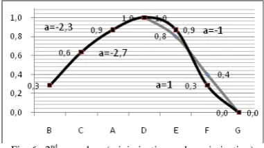
This procedure is applied if we intend to minimize the options criterion attributes to reach an optimal value (in this case option D (14)) but the continuous decrease bellow the optimal value starts to become nefarious.

Fig. 6. 2nd _{procedure (minimization and maximization)}

All the steps of the previous procedure are identical to the ones required to implement this second procedure. There is only a change on the concepts order, when we read maximization on the previous procedure now we should read minimization and vice-versa.

The main changes between the 1st and this 2nd procedure rely on the representation side of the linear and exponential normalization taken as a reference to assess the options to be maximized (this options are compared with the ones on the right side of the graph (see Fig. 6) and on the option to be moved from the position 0 (the option to be adjusted is option B since its intrinsic value is greater than the value of option G – if the value of option B was inferior to the value of option G the 1st procedure should be applied instead of this second one by reversing the S1 column values which leads to the reverse of all the other values).

3rd procedure: options with the same minimum importance value

Maximize options B (2), C (4), A (8), D (10) and minimize options E (14), F (20), G (26) on Table XII.

TABLE XII-3RD PROCEDURE (SAME MINIMUM IMPORTANCE VALUE)

OptionsS 1

Linear norm(x) a

Exp.

norm.Max-Min Multp Denomi-

nator

Exp. Norm. × (Max-Min)

Options value

Linear norm

Max

B 2 0,000 -2 0,000 8 16 128 0,000 32,000 0,052 C 4 0,250 -2 0,455 8 16 128 58,247 90,247 0,146 A 8 0,750 -2 0,898 8 16 128 115,003 147,003 0,238 D 10 1,000 0 1,000 8 16 128 128,000 160,000 0,259

Min

E 14 0,750 2 0,545 16 8 128 69,753 101,753 0,165 F 20 0,375 2 0,175 16 8 128 22,378 54,378 0,088 G 26 0,000 2 0,000 16 8 128 0,000 32,000 0,052

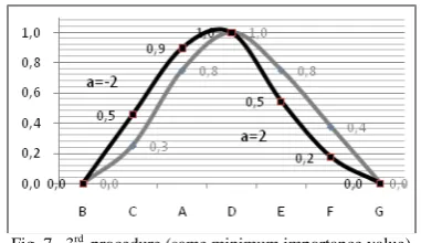
This procedure is applied if we intend to maximize the options criterion attributes but at a specific value the preference starts decreasing and its significance gets as lower as the lowest value we are maximizing (see Fig. 7).

The implementation of this procedure follows the same

any adjustment to the exponential normalization. We just have to define a common denominator for all the options.

Fig. 7. 3rd_{procedure (same minimum importance value)}

On this 3rd procedure we do have both linear and exponential lines on both sides of the graph (see Fig. 7) and we can assess the options symmetry and relative position to determine their actual value according to the decision-maker thoughts and purposes.

V. CONCLUSION AND FURTHER RESEARCH

With the PROV Exponential Decision Method we can actually know, attending to the stakeholders expressions of preference and weights attributed to the options criteria, the exact difference between all the alternatives of solution to attain a certain goal or to solve a problem. The exponential normalization and the processes used to deal with indifference, preference and nefarious values provide a useful framework to analyze tangible and intangible assets and intellectual capital. It would be interesting the development of further work to assess the possible interactions between the proposed decision method and other methods addressing fuzzy and uncertainty inputs.

REFERENCES

[1] J. Canada and W. Sullivan, Economic and Multiattribute Evaluation of Advanced Manufacturing Systems, Prentice Hall, 1989, ch. 10. [2] M. Rogers, Engineering Project Appraisal: the evaluation of

alternative development schemes, Blackwell Science Ltd, 2001. [3] B. Hobbs and P. Meier, Energy decisions and the environment: a

guide to the use of multicriteria methods, Kluwer Academic

Publishers, 2003, pp. 67–98.

[4] F. Figueira and V. Roy, “ELECTRE Methods”, in, M. Ehrgott, J. Figueira and S. Greco, Multiple criteria decision analysis: State of the art surveys, Springer, 2005, pp. 133–162.

[5] J. Brans, J and B. Mareschal, “Promethee methods”, in, M. Ehrgott, J. Figueira and S. Greco. Multiple criteria decision analysis: State of the art surveys, Springer, 2005, pp. 163–195.

[6] M. Matos, Ajuda Multicritério à Decisão – introdução, FEUP, University of Porto, 2005, pp. 15–23.

[7] T. Saaty, “The Analytic Hierarchy and Analytic Network Process for the measurement of intangible criteria and for decision-making”, in, M. Ehrgott, J. Figueira and S. Greco, Multiple criteria decision analysis: State of the art surveys, Springer, 2005, pp. 345–407. [8] N. Munier, A strategy for using multicriteria analysis in

decision-making: A guide for simple and complex environment projects,