Power-Law Adjusted Failure-Time Models

(1)

Power-Law Adjusted Failure-Time Models

William J. Reed

Abstract—A simple adjustment to parametric failure-time distributions, which allows for much greater flexibility in the shape of the hazard-rate function, is considered. Analytical expressions for the distributions of the power-law adjusted Weibull, gamma, log-gamma, generalized gamma, lognormal and Pareto distributions are given. Most of these allow for bathtub shaped and other multi-modal forms of the hazard rate. The new distributions are fitted to real failure-time data which exhibit a multi-modal hazard-rate function and the fits are compared.

Index Terms—survival analysis; bathtub hazard; accelerated failure time (AFT) regression; power-law distribution.

I. INTRODUCTION

Parametric distributions play an important role in the analysis of lifetime data especially in accelerated failure time (AFT) regression models. Generally speaking analysis based on a parametric model will be more precise than that based on a nonparametric or semi-parametric model, because it will have fewer unknown parameters. However this is contingent on it being possible to find a suitable parametric model to fit the data. Unfortunately for most of the common distributions employed there is very little flexibility in the shape of the hazard rate function. In particular none of the two-parameter distributions customarily employed can be used to model a bathtub-shaped hazard.

There are a number of three-parameter distributions which allow a bathtub-shaped hazard including the exponentiated

Weibull[3], thegeneralized Weibull [4] and thegeneralized

gamma(seee.g.[1]) distributions. An addition to these was

proposed in a recent article by Reed [5]. This distribution, which is a special case of adouble Pareto-lognormal distri-bution [6], can be characterised as the product of independent random variables, one with a lognormal distribution and the other with a power-law distribution on[0,1]. For this reason the new distribution was called thelognormal-power function

distribution. It can be thought of as an extension of the lognormal distribution.

In this article it is shown how any simple parametric failure-time distribution can be extended in a similar way to allow for much greater flexibility in its form, including in most cases the possibility of bathtub shaped hazard-rate functions. Precisely, the failure time T is modelled as the

product T =d T0U, where T0 follows the “simple” failure-time distribution and U follows the power-law distribution with density λuλ−1 _on _[0_,_1]_{. Alternatively this can be}

expressed asT =d T0/V whereV has a Pareto distribution,

with densityλ/vλ+1 _on_[1_,

∞).

As might be expected, it is not possible for every paramet-rically specified distribution (of T0) to obtain an analytical

Manuscript received March 9, 2012; revised March, 2012. This work was supported in part by NSERC Grant OGP 7252.

W. J. Reed is emeritus professor at Department of Mathematics and Statistics, University of Victoria, PO Box 3060 STN CSC, Victoria, B.C., Canada V8W 3R4 e-mail:[email protected]

expression for the resulting power-law modified density. However it turns out to be possible to do so for a number of the more common failure-time distributions including the lognormal (Reed, 2011), exponential, Weibull, gamma, log-gamma, Pareto and generalized gamma distributions. These distributions are considered in this article. In all cases, except the lognormal and Pareto, the resulting power-function mod-ified densities can be expressed in terms of an incomplete gamma function.

In Sec.2 the distribution theory associated with the power-law modification is presented, and in Sec.3 maximum likeli-hood estimation discussed. In Sec.4 the results of fitting the various power-law modified failure-time distributions to data with a multi-modal shaped hazard rate, are presented.

II. THEORY

Let T0 be a random variable with a known continuous failure-time distribution. The power-law modified form of this distribution can be represented by a random variable T

with

T =d T0U

whereU, independent of T0, follows the power-law

distri-bution with density λuλ−1 ₍_{λ >} ₀_{) on the interval} _[0_,_1]_.

Taking logarithms leads to

X = log(T)=d Z0−_λ1E

whereZ0= logT0(with survivor function and densityS0(z)

andf0(z), say) andE is a standard (unit mean) exponential

random variable. The survivor function forX can be found as a convolution as follows:

SX(x) = P(Z0−E/λ≥x)

= P(E_≤λ(Z0₋x)) = E{P(E≤λ(Z0−x))|Z0}

= _E{[1₋e−λ(Z0−x)_]_I_[_Z0

−x >0]_}

=

� ∞

x

[1₋e−λ(z−x)]f0(z)dz

= S0(x)−eλx

� ∞

x

e−λzf0(z)dz (1)

where the expectation E is with respect to Z0 and I is a

Bernoulli indicator random variable. Upon integrating by parts one obtains

SX(x) =λeλx

� ∞

x

e−λzS0(z)dz. (2)

From this, by differentiation and using (1), one obtains the corresponding formula for the density ofX

fX(x) =λeλx

� ∞

x

(2)

From (2) and (3) the survivor function and density of T

in terms of those of T0 (ST0(t) and fT0(t)) can be easily

obtained:

ST(t) =λtλ

� ∞

t

u−λ−1ST0(u)du. (4)

fT(t) =λtλ−1

� ∞

t

u−λfT0(u)du. (5)

We now consider power-law modified forms of some specific failure-time distributions.

Weibull and exponential model. If T0 has a Weibull

distribution with hazard rate function hT0(t) = αβt

β−1_{, its}

survivor function and density are ST0(t) = exp(−αt

β₎_and

fT0(t) =αβt

β−1_exp(

−αtβ₎_{. The hazard rate is monotone} increasing for β > 1 and monotone decreasing for β < 1. In the caseβ= 1 it is constant and the Weibull distribution reduces to an exponential distribution. The survivor function and density forZ0= logT0 are

S0(z) = exp(−αeβz) and f0(z) =αβexp(βz−αeβz).

From (2) and (3), the survivor function and density of

X = logT, whereTfollows the power-law adjusted Weibull

distribution, are

SX(x) =

λαλ/β

β e

λx _I₍_αeβx_,

−λ/β)

fX(x) =λαλ/β eλx I(αeβx,1−λ/β)

whereI is the incomplete gamma function

I(y,θ) =

� ∞

y

uθ−1e−udu. (6)

Note that although the ordinary gamma function can be expressed as the integral Γ(θ) = �₀∞uθ−1_e−u_du _{only for}

θ >0, the incomplete gamma function I(y,θ) evaluated at

y >0converges for all realθ. ThusSX(x)andfX(x)above

are well-defined since αeβx_>₀_.

The survivor function, density and hazard-rate function for

T are easily computed from the above as

ST(t) =SX(logt); fT(t) =1

tfX(logt); hT(t) =

fT(t)

ST(t)

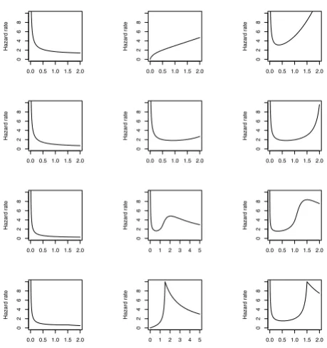
Fig.1 (top row) illustrates three shapes that the hazard rate function of the power-law adjusted Weibull distribution can assume.

Gamma model. If T0 follows a gamma distribution with

scale parameterθ−1 _{and shape parameter}_κ_{, then the density}

and survivor function ofZ0= logT0 are

S0(z) = I(θe

z_{, κ}₎

Γ(κ) and f0(z) =

θκ

Γ(κ)exp(κz−θe

z₎

From (2) and (3), the survivor function and density of

X = logT, whereT follows the power-law adjusted gamma distribution, are

SX(x) = 1

Γ(κ)

�

I(θex, κ)−θλeλxI(θex, κ−λ)�

fX(x) = λθ

λ

Γ(κ) e

λx_I₍_θex_{, κ}

−λ)

0.0 0.5 1.0 1.5 2.0

0 2 4 6 8 Time Hazard rate

0.0 0.5 1.0 1.5 2.0

0 1 2 3 4 5

0.0 0.5 1.0 1.5 2.0

0 2 4 6 8 Hazard rate

0 1 2 3 4 5

0.0 0.5 1.0 1.5 2.0

Fig. 1. Some shapes of the hazard rate function for for various power-law adjusted distributions. Top row: Weibull distribution withα= 1: (l.hand)

β= 1(exponential distribution) andλ= 0.02; (centre)β= 2andλ= 2;

r.handβ= 3andλ=.02. Second row: gamma distribution withθ= 0.25: (l.hand)κ = .01and λ = 1; (centre) κ = .01and λ = 2.5; (r.hand)

κ = .1 and λ = 7. Third row: log-gamma distribution with θ = 20: (l.hand)κ = 50and λ =.01; (centre)κ = 10 andλ =.01; (r.hand)

κ= 5andλ=.5. Bottom row: Pareto distribution withτ0= 1.5: (l.hand) α= 1andλ= 0.1; (centre)α= 15andλ= 2; (r.hand):α= 15and

λ= 0.2

Fig.1 (second row) illustrates some shapes that the hazard rate function of the power-law adjusted gamma distribution can assume.

Log-gamma model. If Z0 = logT0 follows a

gamma distribution, so that T0 has density fT0(t) =

θκ

Γ(κ)t−(θ+1)(logt)κ−1 with support on[1,∞)then from (2)

and (3), it is easy to show that the power-law adjusted random variable T has support on (0,∞) and that X = logT has

survivor function and density

SX(x) =

  

1−eλx�_θ₊θ_λ�

κ

if x≤0

1

Γ(κ)

�

I(θx,κ)₋� θ

θ+λ �κ

eλx_I_([_θ₊_λ_]_x,κ₎� _if _{x >}₀

and

fX(x) =

  

λeλx� θ

θ+λ �κ

ifx_≤0

λeλx� θ

θ+λ

�κ _I_([_θ₊_λ_]_x,κ₎

Γ(κ) ifx >0

Fig.1 (third row) illustrates some shapes that the hazard rate function of the power-law adjusted log-gamma distribution can assume.

Pareto model. If T0 follows a Pareto distribution with

support on(τ0,∞)and pdffT0(t) =

α τ0

� t τ0

�−(α+1)

thereon, one can show that the power-law adjusted form has support on (0,∞)and (using (4)) that the survivor function of the

power-law adjusted form is

ST(t) =

    

1₋_α₊α_λ�_τt₀�λ if t_≤τ0

λ α+λ

� t τ0

�−α

[image:2.595.307.537.59.304.2] [image:2.595.305.537.542.634.2]

(3)

and using (5) that the corresponding pdf is

fT(t) =

    

αλ α+λ

1

τ0

� t τ0

�λ−1

ift≤τ0

αλ α+λ

1

τ0

� t τ0

�−α−1

ift > τ0

Fig.1 (bottom row) illustrates some shapes that the hazard rate function of the power-law adjusted Pareto distribution can assume.

Lognormal model. Consider the case where Z0 = logT0

follows a normal distribution with meanµand varianceσ2_.

Reed (2011) The power-law adjusted version of this distri-bution (the lognormal-power function or lNpf distribution) was considered in [5] where it is shown that the survivor function and density of X = logT, where T follows the lNpf distribution, are

SX(x) =φ

�_x

−µ

σ

� �

R

�_x

−µ

σ

�

−R

�

λσ+x−µ

σ

��

and

fX(x) =λφ

�_x

−µ

σ

�

R

�

λσ+x−µ

σ

�

where R is Mills’ ratio of the complementary cumulative

distribution function (cdf) to the pdf of a standard normal distribution:

R(z) =Φ

c₍_z₎

φ(z).

Generalized gamma model. The three-parameter

general-ized gamma distribution includes the Weibull, gamma and lognormal models as special or limiting cases. It has density

fT0(t) =αθ

κ_tακ−1_exp(

−θtα)/Γ(κ)

With some work using (2) and (3), the survivor function and density of X = logT, where T follows the power-law

adjusted gamma distribution, can be shown to be

SX(x) =

1 Γ(κ)

�

I(θeαx_{, κ}₎

−θλ/α_eλx_I₍_θeαx_{, κ}

−λ/α)�

fX(x) = λθ

λ/α

Γ(κ) e

λx_I₍_θeαx_{, κ}

−λ/α)

It should be noted that while the (unadjusted) log-gamma and Pareto distributions have support bounded away from zero, their power law adjusted versions have support on

[0,∞) as indeed occurs in all of the power law adjusted

models discussed in this paper. Thus in these models there are no problems with the range of support depending on a parameter, as occurs for example with the generalized Weibull distribution.

III. PARAMETER ESTIMATION BY MAXIMUM LIKELIHOOD.

The parametric likelihood for much failure-time data is proportional to

n �

i=1

[fTi(ti)]

δi_[_S

Ti(ti)]

1−δi

whereδiis an indicator variable with value 1 for an observed failure time, and value 0 for a right-censored observation. If there are no covariates and the failure times are considered

0 2000 4000 6000 8000 10000

0e+00

2e

−

04

4e

−

04

6e

−

04

8e

−

04

Time (# of cycles)

[image:3.595.337.511.73.227.2]

Smoothed estimated hazard rate

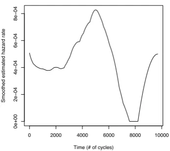
Fig. 2. Kernel smoothed non-parametric estimate of the hazard rate function for electrical appliances data. The Epanechnikov kernel with a bandwith of 1500 was used. Note that the right-hand part (>6000) of the estimated

hazard is unreliable, being based on only two observations.

to be identically distributed following a power-law adjusted distribution with pdf and survivor functionfT andST, then up to an additive constant the log-likelihood is

n �

i=1

δilogfT(ti) +

n �

i=1

(1₋δi) logST(ti)

which is the same as n

�

i=1

δilogfX(logti) +

n �

i=1

(1₋δi) logSX(logti)− n �

i=1

logti

Thus for each of the models discussed above an analytical expression for the log-likelihood can be obtained. This will need to be maximized numerically to obtain maximum likelihood estimates using an optimization routine such as

optiminR. For starting values one can use the MLEs of the two parameters of the unadjusted distribution and an arbitrary value (say 1) forλ.

CovariatesZT _{= (}_{Z1, Z2, . . . , Z}

p)can be incorporated in an accelerated failure time (AFT) regression model:

logT =β0+βT_Z₊_X ₍₇₎ where X is a random variable with one of the

power-law adjusted distributions of the previous section. Note that for all but the log-gamma these distributions can be re-parameterized in terms of a location parameter and two other parameters. In these cases the intercept termβ0 in (7) is not

needed (and indeed will result in a non-identifiable model if it is included).

IV. AN EXAMPLE.

Electrical appliances.Lawless (p. 256) [2] presents data on

(4)

0 2000 4000 6000 8000 10000

0.0000

0.0004

0.0008

0.0012

Time(cycles)

Fitted hazard rate

0 20004000 6000 8000 10000

0.0000

0.0004

0.0008

0.0012

Time(cycles)

Fitted hazard rate

0 2000 4000 6000 8000 10000

0.0000

0.0004

0.0008

0.0012

Time(cycles)

Fitted hazard rate

0 20004000 6000 8000 10000

0.0000

0.0004

0.0008

0.0012

Time(cycles)

[image:4.595.78.253.65.233.2]

Fitted hazard rate

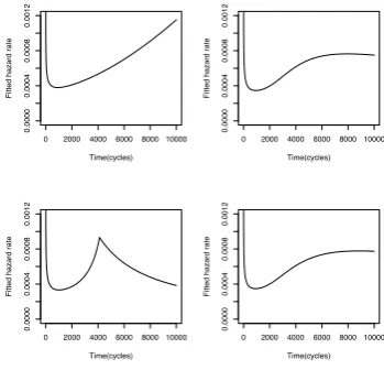
Fig. 3. Maximum likelihood estimates of various power-law adjusted distributions for the electrical appliance data. They are (clockwise from upper left) Weibull, log gamma, lognormal and Pareto.

was performed in Rusing the Nelder-Mead method in the routineoptimand in all cases required only a minute or two of computation.

The values of the maximized log-likelihood and of the Akaike Information Criterion (AIC) for the power-law ad-justed forms of the two-parameter models are given in Table 1. In all cases, the improvement in fit obtained by including the power-law adjustment was highly significant

(P << .001) as one would expect since none of the

[image:4.595.339.505.73.227.2]

two-parameter forms allows for a bathtub shape. From Table 1 it can be seen that the power-law adjusted Pareto distribution provides the best fit of these models.

Fig.3 shows the MLES of the hazard rate for (clockwise from upper left) the power-law adjusted Weibull, log-gamma, lognormal and Pareto distributions. While these plots may appear very different to the non-parametric estimate of the hazard function (Fig.2) at the upper end, it should be noted that the upper part of the non-parametric estimate is not very precise, since in the dataset there are only two observations greater than 6000 (with values 6065 and 9701). Fig.4 shows the fitted power-law adjusted Pareto hazard rate function superimposed on the non-parametric estimate on the range 0 to 6000 cycles. Also Fig.5 shows the Kaplan-Meier estimate of the survivor function and the fitted survivor function for the power-law adjusted Pareto distribution. Both plots suggest a good fit.

Attempts at fitting the four-parameter power-law adjusted generalized gamma distribution were not successful, with different maxima arising with different starting values. This suggests the possibility of identifiability problems with this model. Indeed the generalized gamma distribution without the power-law adjustment is capable of exhibiting a bathtub shaped hazard.

For comparison purposes the three 3-parameter distribu-tions mentioned in the introduction which have been pre-viously used to model data with a bathtub shaped hazard (exponentiated Weibull, generalized Weibull and generalized gamma) were fitted to the electrical appliances data. The results are shown in Table 2. From comparison with Table 1 it can be seen that of all eight models the best fitting is the power-law adjusted Pareto, followed by the

gener-0 1000 2000 3000 4000 5000 6000

0e+00

2e

−

04

4e

−

04

6e

−

04

8e

−

04

1e

−

03

Time (# of cycles)

Estimated hazard rate

0 1000 2000 3000 4000 5000 6000

0e+00

2e

−

04

4e

−

04

6e

−

04

8e

−

04

1e

−

03

Fig. 4. Kernel smoothed non-parametric estimate of the hazard rate function for electrical appliances data and the MLE of the power-law adjusted Pareto hazard-rate.

0 2000 4000 6000 8000 10000

0.0

0.2

0.4

0.6

0.8

1.0

Estimated survival probability

0 2000 4000 6000 8000 10000

0.0

0.2

0.4

0.6

0.8

1.0

Fig. 5. Non-parametric Kaplan-Meier estimate (step function) of the survivor function for the electrical appliance data and the maximum likeli-hood estimate of the survivor function using the power-law adjusted Pareto distribution.

alized Weibull. Furthermore all of the power-law adjusted 2-parameter models, save the Weibull, have a better fit than the generalized gamma and the exponentiated Weibull distributions, suggesting that the consideration of power-law adjusted models may provide a useful addition to the toolkit of practitioners.

V. CONCLUSIONS.

[image:4.595.338.494.294.461.2]

(5)

in evaluating the incomplete gamma functions which occur in the distributions discussed in this paper and so the extra computation involved might not be too great.

REFERENCES

[1] Cox, C., Chu, H., Schneider, M. & Mu˜noz, A. “Parametric survival analysis and taxonomy of hazard functions for the generalized gamma distribution,”’Statist. Med.26, pp. 4352-4374, 2007

[2] Lawless, J. F.Statistical Models and Methods for Lifetime Data.New York: John Wiley and Sons. 1982

[3] Muldholkar, G. S. and D. K. Srivastava, “Exponentiated Weibull family for analyzing bathtub failure-rate data,”’IEEE Trans. Rel., 42, pp. 299-302. 1993

[4] Muldholkar, G. S., Srivastava, D. K. & Kollia, G. D. “A Generalization of the Weibull distribution with application to the analysis of survival data.J. Amer. Stat. Assoc.”’1996. 91, pp. 1575-1583.

[5] Reed, W. J. “A flexible parametric survival model which allows a bathtub shaped hazard rate function”’.J. Appl. Stat.38, 2011. pp. 1665-1680.