Abstract—The need for optimum machining parameters has always been of great concern to the aerospace industry, as the economy of the process largely depends on selecting the best machining parameters for the machine. However, the additional challenge of being environmentally friendly in production while still being cost effective is now imperative. Metal cutting conditions do not always allow companies to reduce the carbon footprint easily. This is particularly pertinent when newer aerospace material such as Boron Carbide Particle Reinforced Aluminium Alloy (AMC220bc) is machined. This material falls under the category of a particulate reinforced Metal Matrix Composite (MMC), where the ceramic fibers disrupt the flow of electrons, resulting in a decrease in thermal conductivity causing the tool interface temperature to increase reducing tool life. This paper will determine the optimum sustainable machining parameters for this material.
Index Terms—Optimum machining parameters, reduced carbon footprint, aerospace material, Taguchi method
I. INTRODUCTION
ircraft parts by necessity should be made from lightweight, durable and fatigue resistant materials. Commonly used aerospace materials which have these qualities are Aluminium alloys, Titanium alloys and Stainless Steels - of which Titanium alloys and Stainless Steels unfortunately have high machinability rating with Aluminium alloys suffering from galling and smearing [1]. Machining notoriously creates waste compelling aerospace companies to reduce their impact on the environment and put in place appropriate waste disposal measures. This in turn is necessitating Life Cycle Analysis (LCA) to be part of all aerospace manufacturing. Companies now need to embrace the sustainable philosophy to reduce their carbon footprint, allowing them to improve their profitability. This requires that the best machining practices are used in an effort to reduce the total amount of greenhouse gas produced during machining. The total waste produced by machining consists of metal chips, tool tips and coolant costs if used. In addition to the obvious waste produced during metal cutting is the amount of greenhouse gas produced from the electrical power used by the machine tool [2]. The technique used for assessing the environmental aspect and potential impact
Manuscript received February18, 2013; revised April 8, 2013. Brian Boswell is a Lecturer at Curtin University, Perth, Western Australia, 6845, corresponding author phone: +61 8 9266 3803; fax: +61 8 9266 2681; (e-mail: b.boswell@ curtin.edu.au)
Mohammad Nazrul Islam is a senior Lecturer at Curtin University, Perth, Western Australia (e-mai
Alokesh Pramanik is a Lecturer at Curtin University, Perth, Western Australia (e-mail: alokesh.pramanik@ curtin.edu.au).
associated with machining is performed in accordance with the Environmental Management Life Cycle Assessment Principles and Framework ISO 14040 standard [3]. This analysis of the machining process identified that the best reduction on greenhouse gasses would be achieved from refining the metal cutting aspect of the process. In practice, many cutting parameters need to be considered, such as cutting force, feed rate, depth of cut, tool path, cutting power, surface finish and tool life [1]. Dry machining is obviously the most ecological form of metal cutting as there are no environmental issues for coolant use or disposal to consider. For this reason the machining tests were all carried out by dry cutting [4]. Machining conditions and parameters are seen to be vital in order to obtain high quality products with the lowest environmental impact, at the lowest cost. The challenge that the aerospace industry faces is how to find the optimum combination of cutting conditions in order to sustainably produce parts at a reduced cost to manufacture. To help achieve this goal Taguchi Method was used to establish the optimum cutting parameters to machine AMC220bc material. This method of statistical control allows the effect of many different machining parameters to be robustly tested on their machining performance. A three level L27 orthogonal array was selected where 0, 1 and 2 represent the different levels of the three control parameters, cutting speed, feed rate and depth of cut.
Analysis of the machining tests provided the deviation and nominal values of the three quality measurements used to determine the optimum sustainable machining parameters (length error, width error and surface roughness). Further analysis implemented the use of signal-to-noise ratios to differentiate the mean value of the experimental and nominal data of these quality measurements. A viable measure of detectability of a flaw is its signal-to-noise ratio (S/N). Signal-to-noise ratio measures how the signal from the defect compares to other background noise [5].
The signal-to-noise ratio classifies quality into three distinct categories and the noise ratio differs with each category. The three different formulas are given below [6];
∑
=−
=
ni i
y
n
N
S
1 2
1
log
10
[dB] (1)
=
22
log
10
s
y
N
S
[dB] (2)
∑
=
−
=
ni i
y
n
N
S
1 2
1
1
log
10
[dB] (3)Sustainable Machining of Aerospace Material
B. Boswell, M. N. Islam,
Member
IAENG,
and A. Pramanik
The results from this formula suggest that the greater the magnitude of the signal-to-noise ratio, the better the result will be because it yields the best quality with least variance [7]. The signal-to-noise ratio for each of the quality measurements; surface roughness, length error and width error were calculated and the mean signal-to-noise ratio for each parameter was found and tabulated. The results were graphed to illustrate the relationship that exists between S/N ratio, and the input parameters at different levels. The gradient of the graph represented the strength of the relationship for each of the machining parameters.
To help analyse the contribution of each variable and their interactions in terms of quality the Pareto ANOVA analysis is implemented. The Pareto ANOVA analysis was completed for each of the quality measures length error, width error and surface roughness. The Pareto ANOVA analysis identified which control parameter affected the quality of the machined workpiece. By using the Pareto principle only 20% of the total machining configuration is now needed to generate 80% of the benefit of completing all machining test configurations [8]. This method separates the total variation of the S/N ratios. Each of the measured quality characteristics length error, width error and surface roughness, has its own S/N values for each of the 27 different tests. In order to obtain accurate result the S/N values are derived from an average value of 3 readings for each of the quality measurements.
II. MACHINE TEST AND SET-UP
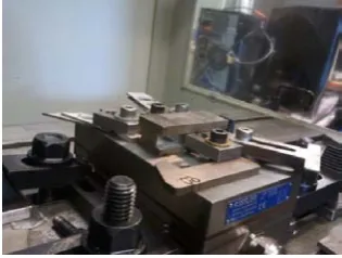
[image:2.595.326.527.55.216.2]Normally a Polycrystalline Diamond (PCD) tool tips is used to machine AMC220bc material as they operate at speeds up to 5000 m/min due to their hardness ~10000mHV and long life. However, uncoated carbide tool tips were used to exhibit the time needed for tool tips to exhibit wear for analysis. Measurement of the cutting forces and power allows for analysis of the cutting operation and optimisation of cutting parameters, as well as identifying wear of the tool tip. These important cutting forces were measured by a Kistler dynamometer which has a high natural frequency, and gives precise measurement. Fig. 1 shows the workpiece securely clamped onto the dynamometer. Dynoware28 software was used to provide high-performance real-time graphics of the cutting forces, and is used for evaluation of the forces.
Fig. 1. Work piece clamped onto dynamometer
[image:2.595.89.247.596.715.2]The end mill used a single tool tip to aid analysis of the cutting action shown in Fig. 2, which typically illustrating the intermittent engagement of the tool tip as it comes in contact with the material.
Fig. 2. Typical cutting forces for end milling
Real time machining power was measured by using a Yokogawa CW140 clamp on a power meter which was attached to the machines input power supply. The physical geometrical characteristics of the workpiece were precisely measured using a Discovery Model D-8 Coordinate Measuring Machine (CMM); the workpieces were split into 3 levels of 9 respectively. Mitutoyo Surftest SJ-201 portable stylus type surface roughness tester was used to measure the surface quality of the workpieces. The ideal roughness represents the best possible finish which can be obtained for a given tool geometry, and feed rate. This can only be achieved if inaccuracies such as chatter are completely eliminated. Natural roughness is greatly influenced by the occurrence of a built up edge. The larger the built up edge, the rougher the surface produced, factors tending to reduce chip-tool friction and to eliminate or reduce the built up edge would yield an improved finish.
dx
x
Y
L
R
L
a
=
∫
0
)
(
1
(4)
For this research there were 27 different combinations of cutting speed, feed rate and depth of cut used, each match up with a trial level in the L27 orthogonal array. The values of the combinations of control parameters that correspond to the L27 orthogonal array can be found from Table I. The best quality measurements will identify the optimal machining parameters for sustainable production. The Leadwell V30 CNC milling machine was used to machine the workpieces, allowing easy changes to the machining parameters for the different tests.
TABLE I
Control Parameters and their Levels
Control
Parameters Units Symbol
Levels Level 0 Level
1
Level 2 Cutting
Speed
m/min A 50 100 150
Feed Rate mm/rev B 0.10 0.20 0.30 Depth of Cut mm C 1.0 1.5 2.0
III. RESULTS AND DISCUSSION
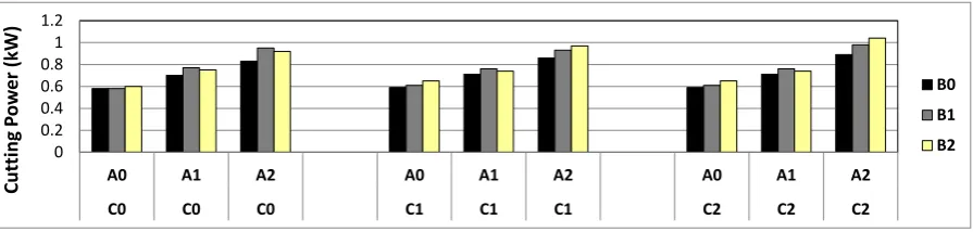
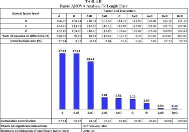
[image:2.595.300.555.660.741.2]different combinations of machining parameters have an effect on quality aspects of the machined workpiece. Variations in cutting power for input parameters; cutting speed, feed rate and depth of cut are shown in Fig. 3 to Fig. 8. In these machining tests an unique combination of control parameters each have different combinations of different level values (0, 1, 2), and machining parameters A, B and C representing the cutting force, feed rate and depth of cut respectively. Table II shows the experimental results and their respective S/N ratios for length, width and surface roughness. For this research the ‘smaller the better’ category of the signal-to-noise ratio is chosen, which is shown as Equation 3. The results from this formula suggest that the greater the magnitude of the signal-to-noise ratio, the better the result will be because it yields the best quality with least variance. Fig. 11 shows that machining parameter with A (cutting speed) having the most significant effect on length error, followed by C (depth of cut) and then B (feed rate). The interaction between A×B also influences the machining process. The lowest depth of cut, C0, was the best depth of cut to achieve a low length error. Since the interaction of A x B was also significant, it can be seen that the optimum combination for factors A and B in order to achieve a low length error was A2B1. Therefore, the combination to help achieve low length error is A2B1C0; i.e., the highest level of cutting speed, medium level of feed rate and low level of depth of cut.
The Pareto ANOVA analysis for length error given in Table III confirms that the parameter that significantly affects the mean length error is cutting speed (with percentage contribution, P = 27.84%). It is worth noting that the interactions A×B, (P = 27.74%) and A×C (P = 23.74%) were more than the main effects for factors B (P = 3.07%) and C (P = 5.13%).Fig. 12 shows that in term of individual effects, machining parameter A (cutting speed) had the most significant effect on width error, followed by C (depth of cut) and then B (feed rate). This stays true with the individual parameter effects on length error. However, when considering all effects, i.e. individual and interaction effects, the interaction between A×C (cutting speed and depth of cut) showed the greatest effect on width error. The medium level of feed rate, B1 (0.2 mm/rev), was the best feed rate to achieve a low width error. Since the interaction of A×C was also significant, it can be seen that the optimum combination for factors A and C in order to achieve a low width error was A1C2. Thus, the optimal combination to achieve the width error was A1B1C2; i.e., the medium level of cutting speed, medium level of feed rate and highest level of depth of cut.
The Pareto ANOVA analysis for width error given in Table IV illustrates that the most significant machining parameter affecting the width error was the interaction between the cutting speed and depth of cut (A×C), (P = 31.33%), followed by cutting speed A (P = 14.49%) and depth of cut C (P = 12.32). Also the total of all interaction effects is higher (P ≅ 66%) than the total of all individual effects (P ≅ 34). Fig. 13 shows that parameter B (feed rate) had the most significant effect on surface roughness, followed by A (cutting speed) and then C (depth of cut). The interaction between B×C also played a role in this machining process. The medium level of cutting speed, A1 (100 m/min), was the best cutting speed to achieve a low surface roughness. Since the interaction of B×C was also significant,
showing that the optimum combination for factors B and C in order to achieve a low surface roughness was B2C0. Therefore, the optimal combination to achieve low surface roughness was A1B2C0; i.e., the medium level of cutting speed, highest level of feed rate and lowest level of depth of cut. The Pareto ANOVA analysis for surface roughness given in Table V confirms that the parameter that significantly affects the mean surface roughness is feed rate (with percentage contribution, P = 77.57%). All other effects, both individual and interaction, had a minimal effect on surface roughness.
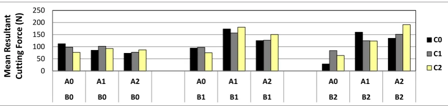
From the analysis of cutting power shown in Fig. 3 to Fig. 8 it can clearly be seen that the feed rate and depth of cut have a minimal independent effect on the cutting power. However, combining the cutting speed and feed rate, or cutting speed and depth of cut increases the required power, showing that the main machining parameter that affects the amount of power required is cutting speed. The mean resultant cutting force in Fig. 9 and Fig. 10 shows that generally a lower depth of cut in combination with a low cutting speed and feed rate generates lower resultant cutting forces. However, feed rate changes the cutting force significantly and its dependence is non-linear. Increasing the cutting speed slightly is found to reduce the cutting force. Cutting speeds at low range tend to form a built-up edge, and disappears at high cutting speeds; the dependence on cutting speed diminishes. Depth of cut also changes the cutting force significantly and the dependence is linear. Varying the depth of cut and the feed rate, yields a method of controlling cutting force [9]. Machining with a positive tool orthogonal rake angle will decrease the cutting force but at the same time increase the possibility of destruction of the tool. Dimensional error can be affected by cutting speed in various ways including increasing thermal distortion, altering tool wear, elastic deformation of the work piece and formation of a built-up edge (BUE).
roughness increased. These effects of cutting speed and depth of cut stay true to the results obtained by [7]. This may have been caused by the plastic deformation of the machined surface from the built-up edge or from the material softening, especially at high temperature and due to dry machining [10]. Although the effects of cutting speed and depth of cut on surface roughness stay true to those found by Rafai and Islam [7], there lies a massive difference in results obtained for feed rate. This research however shows that as the feed rate increases in both increments, the surface roughness decreases respectively each time. This is due to the properties of the metal matrix composite as opposed to conventional steel alloys and carbide materials. The MMC allows for a better surface finish at a faster feed rate, therefore decreasing manufacturing time yet maintaining a better quality product. The results and analyses presented above demonstrate that in end milling of Boron Carbide Particle Reinforced Aluminium Alloy, the cutting parameters, such as cutting speed, feed rate and depth of cut, have significant influences on the quality of the workpiece, i.e. dimensional error in length and width, and surface roughness. However, the results also reveal that strong interaction exists between machining parameters.
IV. CONCLUSION
The experimental investigation has shown that cutting speed affects the power required to cut the material, while feed rate and depth of cut have minimal effects. Feed rate and depth of cut significantly affect cutting force, while cutting speed does minimally. The one machining parameter that seems to affect all three quality measures is feed rate; a fast cut minimises dimensional error and produces a better surface finish. Combining this knowledge with that found from the analysis of the control parameters on quality measurements, it was found that a high feed rate produces a good surface finish, while producing low dimensional errors.
Making the optimum sustainable machining options for this material to be one of high cutting speed with high federate to maximise the material removal rate, showing that Boron Carbide Particle Reinforced Aluminium Alloy can be machined in a sustainable manner. The fact that the surface finish improves with an increase of feed rate is of interest, as this is the opposite found for traditional material being machined this which poses an opportunity for future research.
REFERENCES
[1] T. J. Drozda, C. Wick, J. T. Benedict, R. F. Veilleux, R. Bakerjian, and P. J. Mitchell, Tool and manufacturing engineers handbook : a reference book for manufacturing engineers, managers, and technicians, 4 ed. Michigan: SME Publications, 1983.
[2] T. Gutowski, C. Murphy, D.Allen, D.Bauer, B. Bras, T. Piwonka, P.Sheng, J. Sutherland, D. Thurston, and E. Wolff, "Environmentally Benign Manufacturing: Observations from Japan, Europ and United States," Jounal of Cleaner Production, vol. 13, pp. 1-17, 2005. [3] A. N. I. 14040, "Environmental management Life cycle assessment
Principles and framwork," ed. 1 The Crescent, Homebush NSW 2140 Australia: Standards Australia and Standards New Zealand, 1998. [4] P. S. Sreejith and B. K. A. Ngoi, "Dry machining: Machining of the
future," Journal of Materials Processing Technology, vol. 101, pp. 287-291, 2000.
[5] R. Roy, A Primer on the Taguchi Method: Society of Manufacturing Engineers, 1990.
[6] S. Tanaydin, "Robust Design and Analysis for Quality Engineering," Technometrics, vol. 40, p. 348, 1998.
[7] N. H. Rafai, "An investigation into dimensional accuracy and surface finish achievable in dry turning," Machining science and technology, vol. 13, p. 571, 2009.
[8] D. Haughey. (2013). Pareto Analysis Step by Step. Available:
[9] S. Kalpakjian and S. R. Schmid, Manufacturing Engineering and Technology. Singapore: Prentice Hall, 2010.
[10] R. Azouzi and M. Guillot, "On-line prediction of surface finish and dimensional deviation in turning using neural network based sensor fusion," International Journal of Machine Tools and Manufacture, vol. 37, pp. 1201-1217, 1997
0 0.2 0.4 0.6 0.8 1 1.2
A0 A1 A2 A0 A1 A2 A0 A1 A2
B0 B0 B0 B1 B1 B1 B2 B2 B2
Cut
ti
ng
P
ow
er
(k
W
)
C0 C1 C2
Fig. 3. Comparison of Cutting Power for different levels of cutting speed and feed rate vs. different levels of depth of cut
0 0.2 0.4 0.6 0.8 1 1.2
A0 A1 A2 A0 A1 A2 A0 A1 A2
C0 C0 C0 C1 C1 C1 C2 C2 C2
Cut
ti
ng
P
ow
er
(k
W
)
[image:4.595.76.524.664.771.2]B0 B1 B2
0 0.2 0.4 0.6 0.8 1 1.2
B0 B1 B2 B0 B1 B2 B0 B1 B2
A0 A0 A0 A1 A1 A1 A2 A2 A2
Cut
ti
ng
P
ow
er
(k
W
)
[image:5.595.73.527.84.188.2]C0 C1 C2
Fig. 5. Comparison of Cutting Power for different levels of feed rate and cutting speed vs. different levels of depth of cut
0 0.2 0.4 0.6 0.8 1 1.2
B0 B1 B2 B0 B1 B2 B0 B1 B2
C0 C0 C0 C1 C1 C1 C2 C2 C2
Cut
ti
ng
P
ow
er
(k
W
)
[image:5.595.73.523.217.325.2]A0 A1 A2
Fig. 6. Comparison of Cutting Power for different levels of feed rate and depth of cut vs. different levels of cutting speed
0 0.2 0.4 0.6 0.8 1 1.2
C0 C1 C2 C0 C1 C2 C0 C1 C2
B0 B0 B0 B1 B1 B1 B2 B2 B2
Cut
ti
ng
P
ow
er
(k
W
)
[image:5.595.74.523.352.459.2]A0 A1 A2
Fig. 7. Comparison of Cutting Power for different levels of depth of cut and feed rate vs. different levels of cutting speed
0 0.2 0.4 0.6 0.8 1 1.2
C0 C1 C2 C0 C1 C2 C0 C1 C2
A0 A0 A0 A1 A1 A1 A2 A2 A2
Cut
ti
ng
P
ow
er
(k
W
)
B0 B1 B2
Fig. 8. Comparison of Cutting Power for different levels of depth of cut and cutting speed vs. different levels of feed rate
0 50 100 150 200 250
A0 A1 A2 A0 A1 A2 A0 A1 A2
B0 B0 B0 B1 B1 B1 B2 B2 B2
M
ean
R
es
ult
an
t
Cut
ti
ng
F
or
ce (
N
)
C0 C1 C2
[image:5.595.76.524.486.595.2] [image:5.595.74.522.624.730.2]0 50 100 150 200 250
B0 B1 B2 B0 B1 B2 B0 B1 B2
A0 A0 A0 A1 A1 A1 A2 A2 A2
M
ean
R
es
ult
an
t
Cut
ti
ng
F
or
ce (
N
)
C0 C1 C2
[image:6.595.128.470.285.682.2]Fig. 10. Comparison of Mean Resultant Cutting Force for different levels of feed rate and cutting speed vs. levels of depth of cut
TABLE II
Experimental Results for Length error, Width Error, Surface Roughness and their corresponding S/N Ratios
Measured Parameters Calculated S/N ratio
Ex.No.
Length error (mm)
Width error (mm)
Surface roughness
(µm)
S/N ratio for Length
error
S/N ratio for Width error
S/N ratio for Surface roughness
1 0.34 0.34 5.64 9.40 9.48 -15.02
2 0.21 0.19 3.14 13.45 14.61 -9.93
3 0.30 0.18 2.64 10.34 14.78 -8.43
4 0.22 0.20 1.55 13.03 14.08 -3.83
5 0.21 0.18 1.64 13.43 14.72 -4.28
6 0.30 0.17 2.23 10.38 15.58 -6.98
7 0.23 0.12 1.15 12.96 18.25 -1.25
8 0.35 0.61 1.34 9.12 4.28 -2.51
9 0.19 0.17 1.93 14.26 15.49 -5.71
10 0.21 0.20 2.17 13.47 14.07 -6.71
11 0.24 0.18 2.19 12.24 14.70 -6.82
12 0.29 0.19 2.80 10.64 14.26 -8.95
13 0.23 0.20 1.47 12.87 14.14 -3.36
14 0.24 0.14 1.65 12.32 17.16 -4.34
15 0.34 0.09 1.41 9.47 21.18 -2.96
16 0.26 0.18 1.15 11.60 15.07 -1.18
17 0.36 0.10 1.84 8.83 20.03 -5.30
18 0.21 0.13 1.39 13.46 17.61 -2.84
19 0.17 0.16 3.48 15.32 15.88 -10.83
20 0.21 0.17 2.72 13.36 15.21 -8.69
21 0.29 0.18 2.50 10.71 14.98 -7.97
22 0.18 0.17 1.57 14.83 15.65 -3.93
23 0.17 0.58 1.67 15.24 4.77 -4.45
24 0.22 0.06 2.21 13.20 24.68 -6.87
25 0.27 0.14 1.32 11.30 17.04 -2.43
26 0.20 0.36 1.30 13.96 8.84 -2.25
10.00 12.00 14.00 16.00
A0 A1 A2 B0 B1 B2 C0 C1 C2 0 1 2(AxB)
S
/N
Ra
ti
o
(
d
B)
[image:7.595.110.488.51.198.2]Machining Parameter Level
[image:7.595.110.488.256.520.2]Fig. 11. Response graph for Length Error
TABLE III
Pareto ANOVA Analysis for Length Error
A B AxB AxB C AxC AxC BxC BxC
106.37 108.94 110.34 107.33 114.78 111.53 106.91 103.16 121.12 104.91 114.78 112.68 110.13 111.96 112.07 111.02 121.71 107.96 122.15 109.70 110.40 115.96 106.69 109.82 115.49 108.55 104.34 548.69 60.60 10.67 116.52 101.16 8.24 110.61 546.67 467.87
27.84 3.07 0.54 5.91 5.13 0.42 5.61 27.74 23.74
27.84 55.57 79.31 85.22 90.83 95.97 99.04 99.58 100.00 Check on significant interaction
A2B1C0
Sum at factor level Factor and interaction
0
AxB two-way table Optimum combination of significant factor level
1 2
Sum of squares of difference (S) Contribution ratio (%)
Cumulative contribution
27.84 27.74
23.74
5.91 5.61 5.13
3.07
0.54 0.42
A AxB AxC AxB AxC C B AxB BxC
10.00 12.00 14.00 16.00 18.00
A0 A1 A2 B0 B1 B2 C0 C1 C2 0 1 2(AxC)
S
/N
Ra
ti
o
(
d
B)
Machining Parameter Level
[image:7.595.109.488.560.705.2]TABLE IV
Pareto ANOVA Analysis for Width Error
A B AxB AxB C AxC AxC BxC BxC
121.28 127.97 136.69 121.18 133.66 123.68 137.32 134.02 113.14 148.22 141.96 117.24 143.16 114.32 120.50 135.22 125.45 156.32 121.00 120.57 136.56 126.15 142.51 146.32 117.96 131.03 121.04 1466.94 708.38 751.51 796.61 1247.24 1189.34 677.32 113.51 3171.13
14.49 7.00 7.42 7.87 12.32 11.75 6.69 1.12 31.33
31.33 45.82 58.14 69.89 77.76 85.19 92.19 98.88 100.00 Check on significant interaction
A1B1C2
Sum at factor level Factor and interaction
0
AxC two-way table Optimum combination of significant factor level
1 2
Sum of squares of difference (S) Contribution ratio (%)
Cumulative contribution
31.33
14.49
12.32 11.75
7.87 7.42 7.00 6.69
1.12
AxC A C BxC AxB AxB B AxC BxC
-12.00 -9.00 -6.00 -3.00 0.00
A0 A1 A2 B0 B1 B2 C0 C1 C2 0 1 2(BxC)
S
/N
Ra
ti
o
(
d
B)
[image:8.595.109.487.59.506.2]Machining Parameter Level
[image:8.595.112.487.509.784.2]Fig. 13. Response graph for Surface Roughness
TABLE V
Pareto ANOVA Analysis for Surface Roughness
A B AxB AxB C AxC AxC BxC BxC
-57.94 -83.36 -57.96 -51.05 -48.54 -50.23 -53.72 -59.44 -56.52 -42.46 -41.01 -44.58 -51.91 -48.58 -45.16 -48.67 -47.44 -47.12
-49.76 -25.79 -47.63 -47.21 -53.04 -54.77 -47.78 -43.29 -46.53 359.87 5339.06 295.00 37.61 40.18 138.74 61.75 421.94 188.45
5.23 77.57 4.29 0.55 0.58 2.02 0.90 6.13 2.74
77.57 83.70 88.93 93.22 95.96 97.97 98.87 99.45 100.00 Check on significant interaction
A1B2C0 BxC two-way table Optimum combination of significant factor level
1 2
Sum of squares of difference (S) Contribution ratio (%)
Cumulative contribution
Sum at factor level Factor and interaction
0
77.57
6.13 5.23 4.29 2.74
2.02 0.90 0.58 0.55