Learning Subjective Language

Janyce Wiebe

_{Theresa Wilson}

University of Pittsburgh University of Pittsburgh

Rebecca Bruce

_{Matthew Bell}

University of North Carolina University of Pittsburgh

at Asheville

Melanie Martin

New Mexico State University

Subjectivity in natural language refers to aspects of language used to express opinions, evalua-tions, and speculations. There are numerous natural language processing applications for which subjectivity analysis is relevant, including information extraction and text categorization. The goal of this work is learning subjective language from corpora. Clues of subjectivity are gener-ated and tested, including low-frequency words, collocations, and adjectives and verbs identified using distributional similarity. The features are also examined working together in concert. The features, generated from different data sets using different procedures, exhibit consistency in performance in that they all do better and worse on the same data sets. In addition, this article shows that the density of subjectivity clues in the surrounding context strongly affects how likely it is that a word is subjective, and it provides the results of an annotation study assessing the subjectivity of sentences with high-density features. Finally, the clues are used to perform opinion piece recognition (a type of text categorization and genre detection) to demonstrate the utility of the knowledge acquired in this article.

1. Introduction

Subjectivity in natural language refers to aspects of language used to express opin-ions, evaluatopin-ions, and speculations (Banfield 1982; Wiebe 1994). Many natural lan-guage processing (NLP) applications could benefit from being able to distinguish subjective language from language used to objectively present factual information. Current extraction and retrieval technology focuses almost exclusively on the sub-ject matter of documents. However, additional aspects of a document influence its relevance, including evidential status and attitude (Kessler, Nunberg, Sch ¨utze 1997). Information extraction systems should be able to distinguish between factual infor-mation (which should be extracted) and nonfactual inforinfor-mation (which should be

∗Department of Computer Science, University of Pittsburgh, Pittsburgh, PA 15260. E-mail{wiebe,mbell}@cs.pitt.edu.

†Intelligent Systems Program, University of Pittsburgh, Pittsburgh, PA 15260. Email: [email protected]. ‡Department of Computer Science, University of North Carolina at Asheville, Asheville, NC 28804.

E-mail: [email protected]

§Department of Computer Science, New Mexico State University, Las Cruces, NM 88003. E-mail: [email protected].

discarded or labeled as uncertain). Question-answering systems should distinguish between factual and speculative answers. Multi-perspective question answering aims to present multiple answers to the user based upon speculation or opinions derived from different sources (Carbonell 1979; Wiebe et al. 2003). Multidocument summa-rization systems should summarize different opinions and perspectives. Automatic subjectivity analysis would also be useful to perform flame recognition (Spertus 1997; Kaufer 2000), e-mail classification (Aone, Ramos-Santacruze, and Niehaus 2000), intel-lectual attribution in text (Teufel and Moens 2000), recognition of speaker role in radio broadcasts (Barzialy et al. 2000), review mining (Terveen et al. 1997), review classifi-cation (Turney 2002; Pang, Lee, and Vaithyanathan 2002), style in generation (Hovy 1987), and clustering documents by ideological point of view (Sack 1995). In general, nearly any information-seeking system could benefit from knowledge of how opin-ionated a text is and whether or not the writer purports to objectively present factual material.

To perform automatic subjectivity analysis, good clues must be found. A huge variety of words and phrases have subjective usages, and while some manually de-veloped resources exist, such as dictionaries of affective language (General-Inquirer 2000; Heise 2000) and subjective features in general-purpose lexicons (e.g., the atti-tude adverb features in Comlex [Macleod, Grishman, and Meyers 1998]), there is no comprehensive dictionary of subjective language. In addition, many expressions with subjective usages have objective usages as well, so a dictionary alone would not suffice. An NLP system must disambiguate these expressions in context.

The goal of our work is learning subjective language from corpora. In this article, we generate and test subjectivity clues and contextual features and use the knowledge we gain to recognize subjective sentences and opinionated documents.

Two kinds of data are available to us: a relatively small amount of data manually annotated at the expression level (i.e., labels on individual words and phrases) ofWall Street Journaland newsgroup data and a large amount of data with existing document-level annotations from the Wall Street Journal (opinion pieces, such as editorials and reviews, versus nonopinion pieces). Both are used as training data to identify clues of subjectivity. In addition, we cross-validate the results between the two types of annotation: The clues learned from the expression-level data are evaluated against the document-level annotations, and those learned using the document-level annotations are evaluated against the expression-level annotations.

There were a number of motivations behind our decision to use document-level annotations, in addition to our manual annotations, to identify and evaluate clues of subjectivity. The document-level annotations were not produced according to our annotation scheme and were not produced for the purpose of training and evaluating an NLP system. Thus, they are an external influence from outside the laboratory. In addition, there are a great number of these data, enabling us to evaluate the results on a larger scale, using multiple large test sets. This and cross-training between the two types of annotations allows us to assess consistency in performance of the various identification procedures. Good performance in cross-validation experiments between different types of annotations is evidence that the results are not brittle.

We focus on three types of subjectivity clues. The first are hapax legomena, the set of words that appear just once in the corpus. We refer to them here asunique words. The set of all unique words is a feature with high frequency and significantly higher precision than baseline (Section 3.2).

Interest-ingly, many include noncontent words that are typically on stop lists of NLP systems (e.g.,of, the, get, out, herein the above examples). The method is then used to identify an unusual form of collocation: One or more positions in the collocation may be filled by any word (of an appropriate part of speech) that is unique in the test data.

The third type of subjectivity clue we examine here are adjective and verb fea-tures identified using the results of a method for clustering words according to dis-tributional similarity (Lin 1998) (Section 3.4). We hypothesized that two words may be distributionally similar because they are both potentially subjective (e.g.,tragic,sad, and poignantare identified frombizarre). In addition, we use distributional similarity to improve estimates of unseen events: A word is selected or discarded based on the precision of it together with itsnmost similar neighbors.

We show that the various subjectivity clues perform better and worse on the same data sets, exhibiting an important consistency in performance (Section 4.2).

In addition to learning and evaluating clues associated with subjectivity, we ad-dress disambiguating them in context, that is, identifying instances of clues that are subjective in context (Sections 4.3 and 4.4). We find that the density of clues in the surrounding context is an important influence. Using two types of annotations serves us well here, too. It enables us to use manual judgments to identify parameters for disambiguating instances of automatically identified clues. High-density clues are high precision in both the expression-level and document-level data. In addition, we give the results of a new annotation study showing that most high-density clues are in sub-jective text spans (Section 4.5). Finally, we use the clues together to perform document-level classification, to further demonstrate the utility of the acquired knowledge (Sec-tion 4.6).

At the end of the article, we discuss related work (Section 5) and conclusions (Section 6).

2. Subjectivity

Subjective language is language used to express private states in the context of a text or conversation.Private stateis a general covering term for opinions, evaluations, emotions, and speculations (Quirk et al. 1985). The following are examples of subjective sentences from a variety of document types.

The first two examples are from Usenet newsgroup messages:

(1) I had in mind your facts, buddy, not hers.

(2) Nice touch. “Alleges” whenever facts posted are not in your persona of what is “real.”

The next one is from an editorial:

(3) We stand in awe of the Woodstock generation’s ability to be unceasingly fascinated by the subject of itself. (“Bad Acid,”Wall Street Journal, August 17, 1989)

The next example is from a book review:

The last one is from a news story:

(5) “The cost of health care is eroding our standard of living and sapping industrial strength,” complains Walter Maher, a Chrysler

health-and-benefits specialist. (Kenneth H. Bacon, “Business and Labor Reach a Consensus on Need to Overhaul Health-Care System,”Wall Street Journal, November 1, 1989)

In contrast, the following are examples ofobjective sentences, sentences without sig-nificant expressions of subjectivity:

(6) Bell Industries Inc. increased its quarterly to 10 cents from 7 cents a share.

(7) Northwest Airlines settled the remaining lawsuits filed on behalf of 156 people killed in a 1987 crash, but claims against the jetliner’s maker are being pursued, a federal judge said. (“Northwest Airlines Settles Rest of Suits,”Wall Street Journal, November 1, 1989)

A particular model of linguistic subjectivity underlies the current and past re-search in this area by Wiebe and colleagues. It is most fully presented in Wiebe and Rapaport (1986, 1988, 1991) and Wiebe (1990, 1994). It was developed to support NLP research and combines ideas from several sources in fields outside NLP, especially linguistics and literary theory. The most direct influences on the model were Dolezel (1973) (types of subjectivity clues), Uspensky (1973) (types of point of view), Kuroda (1973, 1976) (pragmatics of point of view), Chatman (1978) (story versus discourse), Cohn (1978) (linguistic styles for presenting consciousness), Fodor (1979) (linguistic description of opaque contexts), and especially Banfield (1982) (theory of subjectivity versus communication).1

The remainder of this section sketches our conceptualization of subjectivity and describes the annotation projects it underlies.

Subjective elementsare linguistic expressions of private states in context. Subjec-tive elements are often lexical (examples arestand in awe,unceasingly,fascinatedin (3) and eroding, sapping, and complainsin (5)). They may be single words (e.g.,complains) or more complex expressions (e.g., stand in awe, what aNP). Purely syntactic or mor-phological devices may also be subjective elements (e.g., fronting, parallelism, changes in aspect).

A subjective element expresses the subjectivity of asource, who may be the writer or someone mentioned in the text. For example, the source of fascinating in (4) is the writer, while the source of the subjective elements in (5) is Maher (according to the writer). In addition, a subjective element usually has a target, that is, what the subjectivity is about or directed toward. In (4), the target is a tale; in (5), the target of Maher’s subjectivity is the cost of health care.

Note our parenthetical above—“according to the writer”—concerning Maher’s subjectivity. Maher is not directly speaking to us but is being quoted by the writer. Thus, the source is anested source, which we notate (writer, Maher); this represents the fact that the subjectivity is being attributed to Maher by the writer. Since sources

are not directly addressed by the experiments presented in this article, we merely illustrate the idea here with an example, to give the reader an idea:

The Foreign Ministry said Thursday that it was “surprised, to put it mildly” by the U.S. State Department’s criticism of Russia’s human rights record and objected in particular to the “odious” section on Chechnya. (Moscow Times, March 8, 2002]

Let us consider some of the subjective elements in this sentence, along with their sources:

surprised, to put it mildly: (writer, Foreign Ministry, Foreign Ministry)

to put it mildly: (writer, Foreign Ministry)

criticism: (writer, Foreign Ministry, Foreign Ministry, U.S. State Department)

objected: (writer, Foreign Ministry)

odious: (writer, Foreign Ministry)

Considersurprised, to put it mildly. This refers to a private state of the Foreign Ministry (i.e., it is very surprised). This is in the context ofThe Foreign Ministry said, which is in a sentence written by the writer. This gives us the three-level source (writer, Foreign Ministry, Foreign Ministry). The phrase to put it mildly, which expresses sarcasm, is attributed to the Foreign Ministry by the writer (i.e., according to the writer, the Foreign Ministry said this). So its source is (writer, Foreign Ministry). The subjective element

criticismhas a deeply nested source: According to thewriter, theForeign Ministrysaid

itis surprised by theU.S. State Department’s criticism.

The nested-source representation allows us to pinpoint the subjectivity in a sen-tence. For example, there is no subjectivity attributed directly to the writer in the above sentence: At the level of the writer, the sentence merely says that someone said something and objected to something (without evaluating or questioning this). If the sentence startedThe magnificent Foreign Ministry said. . ., then we would have an additional subjective element,magnificent, with source (writer).

Note that subjectivedoes not mean not true. Consider the sentenceJohn criticized Mary for smoking. The verbcriticized is a subjective element, expressing negative eval-uation, with nested source (writer, John). But this does not mean that John does not

believe that Mary smokes. (In addition, the fact that John criticized Mary is being presented as true by the writer.)

Similarly,objectivedoes not meantrue. A sentence is objective if the language used to convey the information suggests that facts are being presented; in the context of the discourse, material is objectively presented as if it were true. Whether or not the source truly believes the information, and whether or not the information is in fact true, are considerations outside the purview of a theory of linguistic subjectivity.

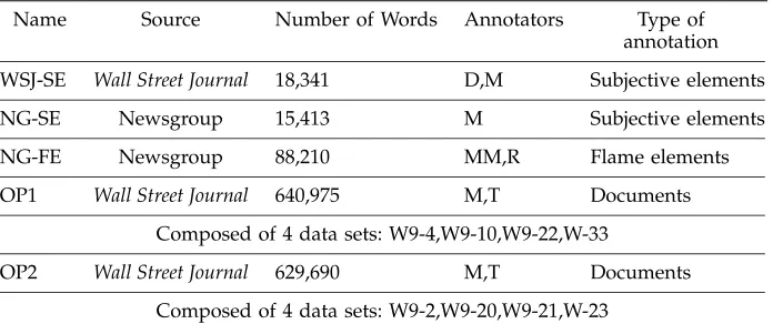
Table 1

Data Sets and Annotations used in Experiments. Annotators M, MM, and T are co-authors of this paper. D and R are not.

Name Source Number of Words Annotators Type of annotation

WSJ-SE Wall Street Journal 18,341 D,M Subjective elements

NG-SE Newsgroup 15,413 M Subjective elements

NG-FE Newsgroup 88,210 MM,R Flame elements

OP1 Wall Street Journal 640,975 M,T Documents

Composed of 4 data sets: W9-4,W9-10,W9-22,W-33

OP2 Wall Street Journal 629,690 M,T Documents

Composed of 4 data sets: W9-2,W9-20,W9-21,W-23

subjectivity. A subjective element is an instance of a potential subjective element, in a particular context, that is indeed subjective in that context (Wiebe 1994).

In this article, we focus on learning lexical items that are associated with subjec-tivity (i.e., PSEs) and then using them in concert to disambiguate instances of them (i.e., to determine whether the instances are subjective elements).

2.1 Manual Annotations

In our subjectivity annotation projects, we do not give the annotators lists of particular words and phrases to look for. Rather, we ask them to label sentences according to their interpretations in context. As a result, the annotators consider a large variety of expressions when performing annotations.

We use data that have been manually annotated at the expression level, the sen-tence level, and the document level. For diversity, we use data from the Wall Street Journal Treebank as well as data from a corpus of Usenet newsgroup messages. Table 1 summarizes the data sets and annotations used in this article. None of the datasets overlap. The annotation types listed in the table are those used in the experiments presented in this article.

In our first subjectivity annotation project (Wiebe, Bruce, and O’Hara 1999; Bruce and Wiebe 1999), a corpus of sentences from the Wall Street Journal Treebank Corpus (Marcus, Santorini, and Marcinkiewicz 1993) (corpus WSJ-SE in Table 1) was annotated at the sentence level by multiple judges. The judges were instructed to classify a sen-tence as subjective if it contained any significant expressions of subjectivity, attributed to either the writer or someone mentioned in the text, and to classify the sentence as objective, otherwise. After multiple rounds of training, the annotators independently annotated a fresh test set of 500 sentences from WSJ-SE. They achieved an average pairwise kappa score of 0.70 over the entire test set, an average pairwise kappa score of 0.80 for the 85% of the test set for which the annotators were somewhat sure of their judgments, and an average pairwise kappa score of 0.88 for the 70% of the test set for which the annotators were very sure of their judgments.

the previous study and asked to put brackets around the words he believed caused the sentence to be classified as subjective.2 _{For example (subjective elements are in}

parentheses):

They paid (yet) more for (really good stuff).

(Perhaps you’ll forgive me) for reposting his response.

No other instructions were given to the annotators and no training was performed for the expression-level task. A single round of tagging was performed, with no commu-nication between annotators. There are techniques for analyzing agreement when an-notations involve segment boundaries (Litman and Passonneau 1995; Marcu, Romera, and Amorortu 1999), but our focus in this article is on words. Thus, our analyses are at the word level: Each word is classified as either appearing in a subjective element or not. Punctuation and numbers are excluded from the analyses. The kappa value for word agreement in this study is 0.42.

Another two-level annotation project was performed in Wiebe et al. (2001), this time involving document-level and expression-level annotations of newsgroup data (NG-FE in Table 1). In that project, we were interested in annotating flames, inflam-matory messages in newsgroups or listservs. Note that inflaminflam-matory language is a kind of subjective language. The annotators were instructed to mark a message as a flame if the main intention of the message is a personal attack and the message contains insulting or abusive language.

After multiple rounds of training, three annotators independently annotated a fresh test set of 88 messages from NG-FE. The average pairwise percentage agreement is 92% and the average pairwise kappa value is 0.78. These results are comparable to those of Spertus (1997), who reports 98% agreement on noninflammatory messages and 64% agreement on inflammatory messages.

Two of the annotators were then asked to identify theflame elementsin the entire corpus NG-FE. Flame elements are the subset of subjective elements that are perceived to be inflammatory. The two annotators were asked to do this in the entire corpus, even those messages not identified as flames, because messages that were not judged to be flames at the document level may contain some individual inflammatory phrases. As above, no training was performed for the expression-level task, and a single round of tagging was performed, without communication between annotators. Agreement was measured in the same way as in the subjective-element study above. The kappa value for flame element annotations in corpus NG-FE is 0.46.

An additional annotation project involved a single annotator, who performed subjective-element annotations on the newsgroup corpus NG-SE.

The agreement results above suggest that good levels of agreement can be achieved at higher levels of classification (sentence and document), but agreement at the expres-sion level is more challenging. The agreement values are lower for the expresexpres-sion-level annotations but are still much higher than that expected by chance.

Note that our word-based analysis of agreement is a tough measure, because it requires that exactly the same words be identified by both annotators. Consider the following example from WSJ-SE:

D: (played the role well) (obligatory ragged jeans a thicket of long hair and rejection of all things conventional)

M: played the role (well) (obligatory) (ragged) jeans a (thicket) of long hair and (rejection) of (all things conventional)

Judge D in the example consistently identifies entire phrases as subjective, while judge M prefers to select discrete lexical items.

Despite such differences between annotators, the expression-level annotations proved very useful for exploring hypotheses and generating features, as described below.

Since this article was written, a new annotation project has been completed. A 10,000-sentence corpus of English-language versions of world news articles has been annotated with detailed subjectivity information as part of a project investigating multiple-perspective question answering (Wiebe et al. 2003). These annotations are much more detailed than the annotations used in this article (including, for example, the source of each private state). The interannotator agreement scores for the new corpus are high and are improvements over the results of the studies described above (Wilson and Wiebe 2003).

The current article uses existing document-level subjective classes, namely edito-rials, letters to the editor,Arts & Leisure reviews, andViewpointsin theWall Street Journal. These are subjective classes in the sense that they are text categories for which subjectivity is a key aspect. We refer to them collectively as opinion pieces. All other types of documents in theWall Street Journalare collectively referred to as nonopinion pieces.

Note that opinion pieces are not 100% subjective. For example, editorials contain objective sentences presenting facts supporting the writer’s argument, and reviews contain sentences objectively presenting facts about the product beign reviewed. Sim-ilarly, nonopinion pieces are not 100% objective. News reports present opinions and reactions to reported events (van Dijk 1988); they often contain segments starting with expressions such as critics claim and supporters argue. In addition, quoted-speech sen-tences in which individuals express their subjectivity are often included (Barzilay et al. 2000). For concreteness, let us consider WSJ-SE, which, recall, has been manually annotated at the sentence level. In WSJ-SE, 70% of the sentences in opinion pieces are subjective and 30% are objective. In nonopinion pieces, 44% of the sentences are subjective and only 56% are objective. Thus, while there is a higher concentration of subjective sentences in opinion versus nonopinion pieces, there are many subjective sentences in nonopinion pieces and objective sentences in opinion pieces.

An inspection of some data reveals that some editorial and review articles are not marked as such by theWall Street Journal. For example, there are articles whose purpose is to present an argument rather than cover a news story, but they are not explicitly labeled as editorials by the Wall Street Journal. Thus, the opinion piece annotations of data sets OP1 and OP2 in Table 1 have been manually refined. The annotation instruc-tions were simply to identify any additional opinion pieces that were not marked as such. To test the reliability of this annotation, two judges independently annotated twoWall Street Journalfiles, W9-22 and W9-33, each containing approximately 160,000 words. This is an “annotation lite” task: With no training, the annotators achieved kappa values of 0.94 and 0.95, and each spent an average of three hours per Wall Street Journal file.

3. Generating and Testing Subjective Features

3.1 Introduction

us-ing the expression-level subjective-element annotations as trainus-ing data, and some are learned using the document-level opinion piece annotations as training data (i.e., opinion piece versus nonopinion piece). All of the clues are evaluated with respect to the document-level opinion piece annotations. While these evaluations are our focus, because many more opinion piece than subjective-element data exist, we do evaluate the clues learned from the opinion piece data on the subjective-element data as well. Thus, we cross-validate the results both ways between the two types of annotations.

Throughout this section, we evaluate sets of clues directly, by measuring the pro-portion of clues that appear in subjective documents or expressions, seeking those that appear more often than expected. In later sections, the clues are used together to find subjective sentences and to perform text categorization.

The following paragraphs give details of the evaluation and experimental design used in this section.

The proportion of clues in subjective documents or expressions is theirprecision. Specifically, the precision of a setS with respect to opinion pieces is

prec(S) = number of instances of members ofSin opinion pieces

total number of instances of members ofSin the data The precision of a setS with respect to subjective elements is

prec(S) =number of instances of members of Sin subjective elements

total number of instances of members ofSin the data

In the above, Sis a set of types (not tokens). The counts are of tokens (i.e., instances or occurrences) of members of S.

Why use a set rather than individual items? Many good clues of subjectivity occur with low frequency (Wiebe, McKeever, and Bruce 1998). In fact, as we shall see below, uniqueness in the corpus is an informative feature for subjectivity classification. Thus, we do not want to discard low-frequency clues, because they are a valuable source of information, and we do not want to evaluate individual low-frequency lexical items, because the results would be unreliable. Our strategy is thus to identify and evaluate sets of words and phrases, rather than individual items.

What kinds of results may we expect? We cannot expect absolutely high precision with respect to the opinion piece classifications, even for strong clues, for three reasons. First, for our purposes, the data are noisy. As mentioned above, while the proportion of subjective sentences is higher in opinion than in nonopinion pieces, the proportions are not 100 and 0: Opinion pieces contain objective sentences, and nonopinion pieces contain subjective sentences.

Second, we are trying to learn lexical items associated with subjectivity, that is, PSEs. As discussed above, many words and phrases with subjective usages have ob-jective usages as well. Thus, even in perfect data with no noise, we would not expect 100% precision. (This is the motivation for the work on density presented in section 4.4.)

Third, the distribution of opinions and nonopinions is highly skewed in favor of nonopinions: Only 9% of the articles in the combination of OP1 and OP2 are opinion pieces.

In this work, increases in precision over a baseline precision are used as evidence that promising sets of PSEs have been found. Our main baseline for comparison is the number of word instances in opinion pieces, divided by the total number of word instances:

Baseline Precision=number of word instances in opinion pieces

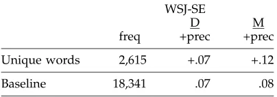
Table 2

Frequencies and increases in precision of unique words in subjective-element data. Baseline frequency is the total number of words, and baseline precision is the proportion of words in subjective elements.

WSJ-SE

D M

freq +prec +prec

Unique words 2,615 +.07 +.12

Baseline 18,341 .07 .08

Words and phrases with higher proportions than this appear more than expected in opinion pieces.

To further evaluate the quality of a set of PSEs, we also perform the following significance test. For a set of PSEs in a given data set, we test the significance of the difference between (1) the proportion of words in opinion pieces that are PSEs and (2) the proportion of words in nonopinion pieces that are PSEs, using the z-significance test for two proportions.

Before we continue, there are a few more technical items to mention concerning the data preparation and experimental design:

• All of the data sets are stemmed using Karp’s morphological analyzer (Karp et al. 1994) and part-of-speech tagged using Brill’s (1992) tagger.

• When the opinion piece classifications are used for training, the existing classifications, assigned by theWall Street Journal, are used. Thus, the processes using them as training data may be applied to more data to learn more clues, without requiring additional manual annotation.

• When the opinion piece data are used for testing, the manually refined classifications (described at the end of Section 2.1) are used.

• OP1 and OP2 together comprise eight treebank files. Below, we often give results separately for the component files, allowing us to assess the consistency of results for the various types of clues.

3.2 Unique Words

In this section, we show that low-frequency words are associated with subjectivity in both the subjective-element and opinion piece data. Apparently, people are creative when they are being opinionated.

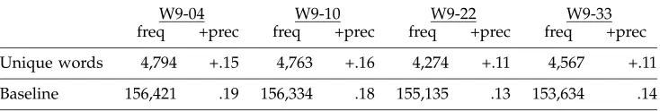
Table 3

Frequencies and increases in precision for words that appear exactly once in the data sets composing OP1. For each data set, baseline frequency is the total number of words, and baseline precision is the proportion of words in opinion pieces.

W9-04 W9-10 W9-22 W9-33

freq +prec freq +prec freq +prec freq +prec

Unique words 4,794 +.15 4,763 +.16 4,274 +.11 4,567 +.11

Baseline 156,421 .19 156,334 .18 155,135 .13 153,634 .14

but the precision of unique words in these same annotations is 0.20, 0.12 points higher than the baseline. This is a 150% improvement over the baseline.

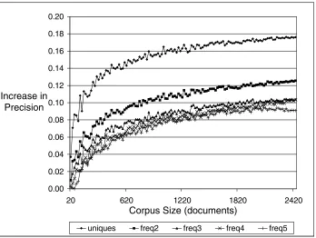
The number of unique words in opinion pieces is also higher than expected. Table 3 compares the precision of the set of unique words to the baseline precision (i.e., the precision of the set of all words that appear in the corpus) in the four WSJ files composing OP1. Before this analysis was performed, numbers were removed from the data (we are not interested in the fact that, say, the number 163,213.01 appears just once in the corpus). The number of words in each data set and baseline precisions are listed at the bottom of the table. Thefreqcolumns give total frequencies. The+preccolumns show the percentage-point improvements in precision over baseline. For example, in W9-10, unique words have precision 0.34: 0.18 baseline plus an improvement over baseline of 0.16. The difference in the proportion of words that are unique in opinion pieces and the proportion of words that are unique in nonopinion pieces is highly significant, withp<0.001 (z≥22) for all of the data sets. Note that not only does the set of unique words have higher than baseline precision, the set is a frequent feature. The question arises, how does corpus size affect the precision of the set of unique words? Presumably, uniqueness in a larger corpus is more meaningful than uniqueness in a smaller one. The results in Figure 1 provide evidence that it is. They-axis in Figure 1 represents increase in precision over baseline and thex-axis represents corpus size. Five graphs are plotted, one for the set of words that appear exactly once (uniques), one for the set of words that appear exactly twice (freq2), one for the set of words that appear exactly three times (freq3), etc.

In Figure 1, increases in precision are given for corpora of size n, where n =

20, 40,. . ., 2420, 2440 documents. Each data point is an average over 25 sample corpora of sizen. The sample corpora were chosen from the concatenation of OP1 and OP2, in which 9% of the documents are opinion pieces. The sample corpora were created by randomly selecting documents from the large corpus, preserving the 9% distribution of opinion pieces. At the smallest corpus size (containing 20 documents), the average number of words is 9,617. At the largest corpus size (containing 2440 documents), the average is 1,225,186 words.

As can be seen in the figure, the precision of unique and other low-frequency words increases with corpus size, with increases tapering off at the largest corpus size tested. Words with frequency 2 also realize a nice increase, although one that is not as dramatic, in precision over baseline. Even words of frequency 3, 4, and 5 show modest increases.

0.00 0.02 0.04 0.06 0.08 0.10 0.12 0.14 0.16 0.18 0.20

20 620 1220 1820 2420

Corpus Size (documents) Increase in

Precision

uniques freq2 freq3 freq4 freq5

Figure 1

Precision of low-frequency words as corpus size increases.

any of our cards are valuable. Only by looking at many packs of cards can we make a determination as to which are the rare ones. Only in samples of sufficient size is uniqueness informative.

The results in this section suggest that an NLP system using uniqueness features to recognize subjectivity should determine uniqueness with respect to the test data augmented with an additional store of (unannotated) data.

3.3 Identifying Potentially Subjective Collocations from Subjective-Element and Flame-Element Annotations

In this section, we describe experiments in identifying potentially subjective colloca-tions.

Collocations are selected from the subjective-element data (i.e., NG-SE, NG-FE, and WSJ-SE), using the union of the annotators’ tags for the data sets tagged by multiple taggers. The results are then evaluated on opinion piece data.

The selection procedure is as follows. First, all 1-grams, 2-grams, 3-grams, and 4-grams are extracted from the data. In this work, each constituent of an n-gram is a word-stem, part-of-speech pair. For example, (in-prep the-det can-noun) is a 3-gram that matches trigrams consisting of preposition in, followed by determiner the, and ending with nouncan.

A subset of then-grams are then selected based on precision. The precision of an

n-gram is the number of subjective instances of that n-gram in the data divided by the total number of instances of thatn-gram in the data. An instance of ann-gram is subjective if each word occurs in a subjective element in the data.

are in subjective elements). Second, the precision of then-gram must be greater than the maximum precision of its constituents. This criterion is used to avoid selecting unnecessarily long collocations. For example,scumbagis a strongly subjective clue. If

be a scumbag does not have higher precision than scumbag alone, we do not want to select it.

Specifically, let (W1,W2) be a bigram consisting of consecutive wordsW1 andW2. (W1,W2) is identified as a potential subjective element ifprec(W1,W2)≥0.1 and:

prec(W1,W2)>max(prec(W1),prec(W2))

For trigrams, we extend the second condition as follows. Let (W1,W2,W3) be a trigram consisting of consecutive wordsW1,W2, andW3. The condition is then

prec(W1,W2,W3)>max(prec(W1,W2),prec(W3))

or

prec(W1,W2,W3)>max(prec(W1),prec(W2,W3))

The selection of 4-grams is similar to the selection of 3-grams, comparing the 4-gram first with the maximum of the precisions of wordW1 and trigram (W2,W3,W4) and then with the maximum of the precisions of trigram (W1,W2,W3) and wordW4. We call the n-gram collocations identified as above fixed-n-grams.

We also define a type of collocation called aunique generalizedn-gram (ugen-n -gram). Such collocations have placeholders for unique words. As will be seen below, these are our highest-precision features.

To find and select such generalized collocations, we first find every word that appears just once in the corpus and replace it with a new word, UNIQUE (but re-membering the part of speech of the original word). In essence, we treat the set of single-instance words as a single, frequently occurring word (which occurs with var-ious parts of speech). Precisely the same method used for extracting and selecting

n-grams above is used to obtain the potentially subjective collocations with one or more positions filled by a UNIQUE, part-of-speech pair.

To test the ugen-n-grams extracted from the subjective-element training data using the method outlined above, we assess their precision with respect to opinion piece data. As with the training data, all unique words in the test data are replaced by

UNIQUE. When a ugen-n-gram is matched against the test data, the UNIQUEfillers match words (of the appropriate parts of speech) that are unique in the test data.

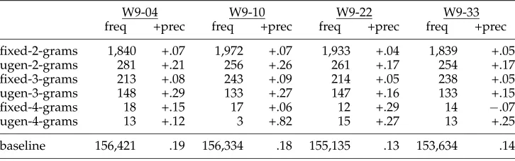
Table 4 shows the results of testing the fixed-n-gram and the ugen-n-gram patterns identified as described above on the four data sets composing OP1. Thefreq columns give total frequencies, and the +prec columns show the improvements in precision from the baseline. The number of words in each data set and baseline precisions are given at the bottom of the table. For alln-gram features besides the fixed-4-grams and ugen-4-grams, the proportion of features in opinion pieces is significantly greater than the proportion of features in nonopinion pieces.3

The question arises, how much overlap is there between instances of fixed-n-grams and instances of ugen-n-grams? In the test data of Table 4, there are a total of 8,577 fixed-n-grams instances. Only 59 of these, fewer than 1% are contained (wholly or in part) in ugen-n-gram instances. This small intersection set shows that two different types of potentially subjective collocations are being recognized.

Table 4

Frequencies and increases in precision of fixed-n-gram and ugen-n-gram collocations learned from the subjective-element data. For each data set, baseline frequency is the total number of words, and baseline precision is the proportion of words in opinion pieces.

W9-04 W9-10 W9-22 W9-33

freq +prec freq +prec freq +prec freq +prec

fixed-2-grams 1,840 +.07 1,972 +.07 1,933 +.04 1,839 +.05

ugen-2-grams 281 +.21 256 +.26 261 +.17 254 +.17

fixed-3-grams 213 +.08 243 +.09 214 +.05 238 +.05

ugen-3-grams 148 +.29 133 +.27 147 +.16 133 +.15

fixed-4-grams 18 +.15 17 +.06 12 +.29 14 −.07

ugen-4-grams 13 +.12 3 +.82 15 +.27 13 +.25

baseline 156,421 .19 156,334 .18 155,135 .13 153,634 .14

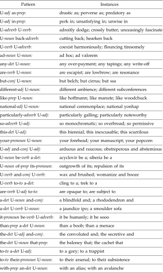
Randomly selected examples of our learned collocations that appear in the test data are given in Tables 5 and 6. It is interesting to note that the unique generalized collocations were learned from the training data by their matching different unique words from the ones they match in the test data.

3.4 Generating Features from Document-Level Annotations Using Distributional Similarity

In this section, we identify adjective and verb PSEs using distributional similarity. Opinion-piece data are used for training, and (a different set of) opinion-piece data and the subjective-element data are used for testing.

Withdistributional similarity, words are judged to be more or less similar based on their distributional patterning in text (Lee 1999; Lee and Pereira 1999). Our

Table 5

Random sample of fixed-3-gram collocations in OP1.

one-nounof-prephis-det worst-adjof-prepall-det

quality-nounof-prepthe-det to-prepdo-verbso-adverb

in-prepthe-detcompany-noun you-pronounand-conjyour-pronoun

have-verbtaken-verbthe-det rest-nounof-prepus-pronoun

are-verbat-prepleast-adj but-conjif-prepyou-pronoun

as-prepa-detweapon-noun continue-verbto-todo-verb

purpose-nounof-prepthe-det could-modalhave-verbbe-verb

it-pronounseem-verbto-prep to-pronouncontinue-verbto-prep

have-verbbe-verbthe-det do-verbsomething-nounabout-prep

cause-verbyou-pronounto-to evidence-nounto-toback-adverb

that-prepyou-pronounare-verb i-pronounbe-verbnot-adverb

Table 6

Random sample of unique generalized collocations in OP1.U:UNIQUE.

Pattern Instances

U-adjas-prep: drastic as; perverse as; predatory as

U-adjin-prep: perk in; unsatisfying in; unwise in

U-adverbU-verb: adroitly dodge; crossly butter; unceasingly fascinate

U-nounback-adverb: cutting back; hearken back

U-verbU-adverb: coexist harmoniously; flouncing tiresomely

ad-nounU-noun: ad hoc; ad valorem

any-detU-noun: any over-payment; any tapings; any write-off

are-verbU-noun: are escapist; are lowbrow; are resonance

but-conjU-noun: but belch; but cirrus; but ssa

different-adjU-noun: different ambience; different subconferences

like-prepU-noun: like hoffmann; like manute; like woodchuck

national-adjU-noun: national commonplace; national yonhap

particularly-adverbU-adj: particularly galling; particularly noteworthy

so-adverbU-adj: so monochromatic; so overbroad; so permissive

this-detU-adj: this biennial; this inexcusable; this scurrilous

your-pronounU-noun: your forehead; your manuscript; your popcorn

U-adjand-conjU-adj: arduous and raucous; obstreperous and abstemious

U-nounbe-verba-det: acyclovir be a; siberia be a

U-nounof-prepits-pronoun: outgrowth of its; repulsion of its

U-verband-conjU-verb: wax and brushed; womanize and booze

U-verbto-toa-det: cling to a; trek to a

are-verbU-adjto-to: are opaque to; are subject to

a-detU-nounand-conj: a blindfold and; a rhododendron and

a-detU-verbU-noun: a jaundice ipo; a smoulder sofa

it-pronounbe-verbU-adverb: it be humanly; it be sooo

than-prepa-detU-noun: than a boob; than a menace

the-detU-adjand-conj: the convoluted and; the secretive and

the-detU-nounthat-prep: the baloney that; the cachet that

to-toa-detU-adj: to a gory; to a trappist

to-totheir-pronounU-noun: to their arsenal; to their subsistence

trainingPrec(s)is the precision ofsin the training data

validationPrec(s)is the precision ofsin the validation data

testPrec(s)is the precision ofsin the test data (similarly fortrainingFreq,validationFreq, andtestFreq)

S = the set of all adjectives (verbs) in the training data forT in [0.01,0.04,. . .,0.70]:

fornin [2,3,. . .,40]:

retained={}

For siinS:

iftrainingPrec({si} ∪Ci,n)>T:

retained=retained∪ {si} ∪Ci,n

RT,n=retained

ADJpses={}(VERBpses ={})

forT in [0.01,0.04,. . .,0.70]: fornin [2,3,. . .,40]:

if validationPrec(RT,n)≥0.28 (0.23 for verbs) and validationFreq(RT,n)≥100:

ADJpses=ADJpses∪RT,n (VERBpses=VERBpses∪RT,n)

Results in Table 7 showtestPrec(ADJpses)andtestFreq(ADJpses). Figure 2

Algorithm for selecting adjective and verb features using distributional similarity.

motivation for experimenting with it to identify PSEs was twofold. First, we hypoth-esized that words might be distributionally similar because they share pragmatic us-ages, such as expressing subjectivity, even if they are not close synonyms. Second, as shown above, low-frequency words appear more often in subjective texts than ex-pected. We did not want to discard all low-frequency words from consideration but cannot effectively judge the suitability of individual words. Thus, to decide whether to retain a word as a PSE, we consider the precision not of the individual word, but of the word together with a cluster of words similar to it.

Many variants of distributional similarity have been used in NLP (Lee 1999; Lee and Pereira 1999). Dekang Lin’s (1998) method is used here. In contrast to many implementations, which focus exclusively on verb-noun relationships, Lin’s method incorporates a variety of syntactic relations. This is important for subjectivity recogni-tion, because PSEs are not limited to verb-noun relationships. In addirecogni-tion, Lin’s results are freely available.

A set of seed words begins the process. For each seedsi, the precision of the set

{si}∪Ci,nin the training data is calculated, whereCi,nis the set ofnwords most similar

to si, according to Lin’s (1998) method. If the precision of {si} ∪Ci,n is greater than a

thresholdT, then the words in this set are retained as PSEs. If it is not, neithersinor the words inCi,nare retained. The union of the retained sets will be denotedRT,n, that is, the union of all sets{si} ∪Ci,nwith precision on the training set>T.

In Wiebe (2000), the seeds (the sis) were extracted from the subjective-element annotations in corpus WSJ-SE. Specifically, the seeds were the adjectives that appear at least once in a subjective element in WSJ-SE. In this article, the opinion piece corpus is used to move beyond the manual annotations and small corpus of the earlier work, and a much looser criterion is used to choose the initial seeds: All of the adjectives (verbs) in the training data are used.

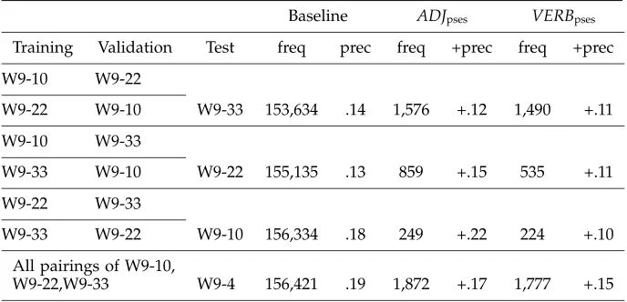
Table 7

Frequencies and increases in precision for adjective and verb features identified using distributional similarity with filtering. For each test data set, baseline frequency is the total number of words, and baseline precision is the proportion of words in opinion pieces.

Baseline ADJpses VERBpses

Training Validation Test freq prec freq +prec freq +prec

W9-10 W9-22

W9-22 W9-10 W9-33 153,634 .14 1,576 +.12 1,490 +.11

W9-10 W9-33

W9-33 W9-10 W9-22 155,135 .13 859 +.15 535 +.11

W9-22 W9-33

W9-33 W9-22 W9-10 156,334 .18 249 +.22 224 +.10

All pairings of W9-10,

W9-22,W9-33 W9-4 156,421 .19 1,872 +.17 1,777 +.15

adjectives versus 0.23 for verbs. These thresholds were determined using validation data.

Seeds and their clusters are assessed on a training set for many parameter settings (cluster size n from 2 through 40, and precision threshold T from 0.01 through 0.70 by .03). As mentioned above, each(n,T)parameter pair yields a set of adjectivesRT,n,

that is, the union of all sets{si} ∪Ci,nwith precision on the training set>T. A subset,

ADJpses, of those sets is chosen based on precision and frequency in a validation set.

Finally, theADJpses are tested on the test set.

Table 7 shows the results for four opinion piece test sets. Multiple training-validation data set pairs are used for each test set, as given in Table 7. The results are for the union of the adjectives (verbs) chosen for each pair. Thefreqcolumns give total frequencies, and the +prec columns show the improvements in precision from the baseline. For each data set, the difference between the proportion of instances of ADJpses in opinion pieces and the proportion in nonopinion pieces is significant

(p<0.001,z≥9.2). The same is true forVERBpses (p<0.001,z≥4.1).

In the interests of testing consistency, Table 8 shows the results of assessing the adjective and verb features generated from opinion piece data (ADJpses andVERBpses

Table 8

Average frequencies and increases in precision in subjective-element data of the sets tested in Table 7. The baselines are the precisions of

adjectives/verbs that appear in subjective elements in the subjective-element data.

Adj baseline Verb baseline ADJpses VERBpses freq prec freq prec freq +prec freq +prec

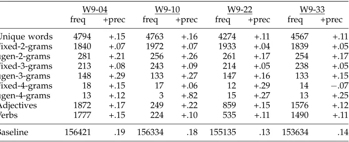
Table 9

Frequencies and increases in precision for all features. For each data set, baseline frequency is the total number of words, and baseline precision is the proportion of words in opinion pieces. freq: total frequency; +prec: increase in precision over baseline.

W9-04 W9-10 W9-22 W9-33

freq +prec freq +prec freq +prec freq +prec

Unique words 4794 +.15 4763 +.16 4274 +.11 4567 +.11 Fixed-2-grams 1840 +.07 1972 +.07 1933 +.04 1839 +.05

ugen-2-grams 281 +.21 256 +.26 261 +.17 254 +.17

Fixed-3-grams 213 +.08 243 +.09 214 +.05 238 +.05

ugen-3-grams 148 +.29 133 +.27 147 +.16 133 +.15

Fixed-4-grams 18 +.15 17 +.06 12 +.29 14 −.07

ugen-4-grams 13 +.12 3 +.82 15 +.27 13 +.25

Adjectives 1872 +.17 249 +.22 859 +.15 1576 +.12

Verbs 1777 +.15 224 +.10 535 +.11 1490 +.11

Baseline 156421 .19 156334 .18 155135 .13 153634 .14

in Table 7) on the subjective-element data. The left side of the table gives baseline figures for each set of subjective-element annotations. The right side of the table gives the average frequencies and increases in precision over baseline for the ADJpses and

VERBpses sets on the subjective-element data. The baseline figures in the table are the

frequencies and precisions of the sets of adjectives and verbs that appear at least once in a subjective element. Since these sets include words that appear just once in the corpus (and thus have 100% precision), the baseline precision is a challenging one.

Testing theVERBpsesandADJpseson the subjective-element data reveals some

inter-esting consistencies for these subjectivity clues. The precision increases of theVERBpses

on the subjective-element data are comparable to their increases on the opinion piece data. Similarly, the precision increases of the ADJpses on the subjective-element data

are as good as or better than the performance of this set of PSEs on the opinion piece data. Finally, the precisions increases for theADJpses are higher than for theVERBpses

on all data sets. This is again consistent with the higher performance of the ADJpses

sets in the opinion piece data sets.

4. Features Used in Concert

4.1 Introduction

In this section, we examine the various types of clues used together. In preparation for this work, all instances in OP1 and OP2 of all of the PSEs identified as described in Section 3 have been automatically identified. All training to define the PSE instances in OP1 was performed on data separate from OP1, and all training to define the PSE instances in OP2 was performed on data separate from OP2.

4.2 Consistency in Precision among Data Sets

0.PSEs = all adjs, verbs, modals, nouns, and adverbs that appear at least once in anSE(except not,will,be,have).

1.PSEinsts= the set of all instances ofPSEs

2.HiDensity={} 3. ForPinPSEinsts:

4.leftWin(P) = theW words beforeP

5.rightWin(P) = theW words afterP

6.density(P) = number of SEswhose first or last word is in leftWin(P) or rightWin(P) 7. ifdensity(P)≥T:

HiDensity=HiDensity∪ {P}

8.prec(PSEinsts) =number of PSEinsts_|PSEinstsin subject elements_|

9.prec(HiDensity) = number ofHiDensity_|HiDensityin subject elements_|

Figure 3

Algorithm for calculating density in subjective-element data.

adjectives and verbs were generated from WSJ document-level opinion piece classifi-cations; then-gram features were generated from newsgroup and WSJ expression-level subjective-element classifications; and the unique unigram feature requires no training. This consistency in performance suggests that the results are not brittle.

4.3 Choosing Density Parameters from Subjective-Element Data

In Wiebe (1994), whether a PSE is interpreted to be subjective depends, in part, on how subjective the surrounding context is. We explore this idea in the current work, assessing whether PSEs are more likely to be subjective if they are surrounded by sub-jective elements. In particular, we experiment with a density feature to decide whether or not a PSE instance is subjective: If a sufficient number of subjective elements are nearby, then the PSE instance is considered to be subjective; otherwise, it is discarded. The density parameters are a window sizeWand a frequency thresholdT.

In this section, we explore the density of manually annotated PSEs in subjective-element data and choose density parameters to use in Section 4.4, in which we apply them to automatically identified PSEs in opinion piece data.

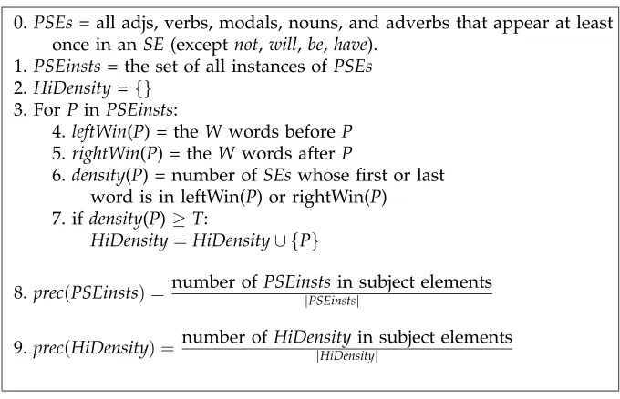
The process for calculating density in the subjective-element data is given in Fig-ure 3. The PSEs are defined to be all adjectives, verbs, modals, nouns, and adverbs that appear at least once in a subjective element, with the exception of some stop words (line 0 of Figure 3). Note that these PSEs depend only on the subjective-element man-ual annotations, not on the automatically identified features used elsewhere in the article or on the document-level opinion piece classes. PSEinsts is the set of PSE instances to be disambiguated (line 1). HiDensity (initialized on line 2) will be the subset of PSEinsts that are retained. In the loop, the density of each PSE instance

P is calculated. This is the number of subjective elements that begin or end in the

W words preceding or following P (line 6). P is retained if its density is at least T

(line 7).

Table 10

Most frequent entry in the top three precision intervals for each subjective-element data set.

WSJ-SE1-M WSJ-SE1-D WSJ-SE2-M WSJ-SE2-D NG-SE

Baseline freq 1,566 1,245 1,167 1,108 3,303

Baseline prec .49 .47 .41 .36 .51

Range .87–.92 .95–1.0 .95–1.0 .95–1.0 .95–1.0

T, W 10, 20 12, 50 20, 50 14, 100 10, 10

freq 76 12 1 1 3

prec .89 1.0 1.0 1.0 1.0

Range .82–.87 .90–.95 .73–.78 .51–.56 .67–.72

T, W 6, 10 12, 60 46, 190 22, 370 26, 90

freq 63 22 53 221 664

prec .84 .91 .78 .51 .67

Range .77–.82 .84–.89 .66–.71 .46–.51 .63–.67

T, W 12, 40 12, 80 18, 60 16, 310 8, 30

freq 292 42 53 358 1504

prec .78 .88 .68 .47 .63

there is evidence that the number of subjective elements near a PSE instance is related to its subjectivity in context.

To create more data points for this analysis, WSJ-SE was split into two (WSJ-SE1 and WSJ-SE2) and annotations of the two judges are considered separately. WSJ-SE2-D, for example, refers to D’s annotations of WSJ-SE2. The process in Figure 3 was repeated for different parameter settings (Tin[1, 2, 4,. . ., 48]andWin[1, 10, 20,. . ., 490]) on each of the SE data sets. To find good parameter settings, the results for each data set were sorted into five-point precision intervals and then sorted by frequency within each interval. Information for the top three precision intervals for each data set are shown in Table 10, specifically, the parameter values (i.e., T and W) and the frequency and precision of the most frequent result in each interval. The intervals are in the rows labeledRange. For example, the top three precision intervals for WSJ-SE1-M, 0.87-0.92, 0.82-0.87, and 0.77-0.82 (no parameter values yield higher precision than 0.92). The top of Table 10 gives baseline frequencies and precisions, which are |PSEinsts| and

prec(PSEinsts), respectively, in line 8 of Figure 3.

The parameter values exhibit a range of frequencies and precisions, with the ex-pected trade-off between precision and frequency. We choose the following parameters to test in Section 4.4: For each data set, for each precision interval whose lower bound is at least 10 percentage points higher than the baseline for that data set, the top two (T,W) pairs yielding the highest frequencies in that interval are chosen. Among the five data sets, a total of 45 parameter pairs were so selected. This exercise was completed once, without experimenting with different parameter settings.

4.4 Density for Disambiguation

0.PSEinsts= the set of instances in the test data of all PSEs described in Section 3 1.HiDensity={}

2. ForPinPSEinsts:

3.leftWin(P) = theW words beforeP

4.rightWin(P) = theW words afterP

5.density(P) = number of PSEinstswhose first or last word is in leftWin(P) or rightWin(P)

6. ifdensity(P)≥T:

HiDensity=HiDensity∪ {P}

7.prec(PSEinsts) =# of PSEinsts_|PSEinsts|inOPs

8.prec(HiDensity) = # ofHiDensity_|HiDensity|inOPs

Figure 4

Algorithm for calculating density in opinion piece (OP) data

number of other PSE instances nearby, wherePSEinstsconsists of all instances of the automatically identified PSEs described in Section 3, for which results are given in Table 9.

Second, in Figure 4, we assess precision with respect to the document-level classes (lines 7–8). The test data are OP1.

An interesting question arose when we were defining the PSE instances: What should be done with words that are identified to be PSEs (or parts of PSEs) according to multiple criteria? For example, sunny, radiant, and exhilarating are all unique in corpus OP1, and are all members of the adjective PSE feature defined for testing on OP1. Collocations add additional complexity. For example, consider the sequence

and splendidly, which appears in the test data. The sequence and splendidly matches the ugen-2-gram (and-conj U-adj), and the word splendidly is unique. In addition, a sequence may match more than one n-gram feature. For example, is it that matches three fixed-n-gram features:is it,is it that, andit that.

In the current experiments, the more PSEs a word matches, the more weight it is given. The hypothesis behind this treatment is that additional matches represent additional evidence that a PSE instance is subjective. This hypothesis is realized as follows: Each match of each member of each type of PSE is considered to be a PSE instance. Thus, among them, there are 11 members in PSEinsts for the five phrases

sunny, radiant, exhilarating, and splendidly, and is it that, one for each of the matches mentioned above.

The process in Figure 4 was conducted with the 45 parameter pair values (T and

W) chosen from the subjective-element data as described in Section 4.3. Table 11 shows results for a subset of the 45 parameters, namely, the most frequent parameter pair chosen from the top three precision intervals for each training set. The bottom of the table gives a baseline frequency and a baseline precision in OP1, defined as|PSEinsts|

andprec(PSEinsts), respectively, in line 7 of Figure 4.

Table 11

Results for high-density PSEs in test dataOP1 using parameters chosen from subjective-element data.

WSJ-SE1-M WSJ-SE1-D WSJ-SE2-M WSJ-SE2-D NG-SE

T, W 10, 20 12, 50 20, 50 14, 100 10, 10

freq 237 3,176 170 10,510 8

prec .87 .72 .97 .57 1.0

T, W 6, 10 12, 60 46, 190 22, 370 26, 90

freq 459 5,289 1,323 21,916 787

prec .68 .68 .95 .37 .92

T, W 12, 40 12, 80 18, 60 16, 310 8, 30

freq 1,398 9,662 906 24,454 3,239

prec .79 .58 .87 .34 .67

PSE baseline: freq = 30,938, prec = .28

and 199%, and 38% yield increases between 22% and 99%. In addition, the increases are significant. Using the set of high-density PSEs defined by the parameter pair with the least increase over baseline, we tested the difference in the proportion of PSEs in opinion pieces that are high-density and the proportion of PSEs in nonopinion pieces that are high-density. The difference between these two proportions is highly significant (z=46.2,p<0.0001).

Notice that, except for one blip (T,W = 6, 10 under WSJ-SE-M), the precisions decrease and the frequencies increase as we go down each column in Table 11. The same pattern can be observed with all 45 parameter pairs (results not included here because of space considerations). But the parameter pairs are ordered in Table 11 based on performance in the manually annotated subjective-element data, not based on performance in the test data. For example, the entry in the first row, first column (T,W=10, 20) is the parameter pair giving the highest frequency in the top precision interval of WSJ-SE-M (frequency and precision in WSJ-SE-M, using the process of Figure 3). Thus, the relative precisions and frequencies of the parameter pairs are carried over from the training to the test data. This is quite a strong result, given that the PSEs in the training data are from manual annotations, while the PSEs in the test data are our automatically identified features.

4.5 High-Density Sentence Annotations

To assess the subjectivity of sentences with high-density PSEs, we extracted the 133 sentences in corpus OP2 that contain at least one high-density PSE and manually annotated them. We refer to these sentences as the system-identifiedsentences.

We chose the density-parameter pair (T,W = 12, 30), based on its precision and frequency in OP1. This parameter setting yields results that have relatively high pre-cision and low frequency. We chose a low-frequency setting to make the annotation study feasible.

Table 12

Examples of system-identified sentences.

(1) The outburst of shooting came nearly two weeks after clashes between Moslem worshippers and oo Somali soldiers.

(2.a) But now the refugees are streaming across the border and alarming the world. ss (2.b) In the middle of the crisis, Erich Honecker was hospitalized with a gall stone operation. oo (2.c) It is becoming more and more obvious that his gallstone-age communism is dying with him:. . . ss

(3.a) Not brilliantly, because, after all, this was a performer who was collecting paychecks from lounges ss at Hiltons and Holiday Inns, but creditably and with the air of someone for whom

“Ten Cents a Dance” was more than a bit autobiographical.

(3.b) “It was an exercise of blending Michelle’s singing with Susie’s singing,” explained Ms. Stevens. oo

(4) Enlisted men and lower-grade officers were meat thrown into a grinder. ss

(5) “If you believe in God and you believe in miracles, there’s nothing particularly crazy about that.” ss

(6) He was much too eager to create “something very weird and dynamic,” ss “catastrophic and jolly” like “this great and coily thing” “Lolita.”

(7) The Bush approach of mixing confrontation with conciliation strikes some people as sensible, perhaps ss even inevitable, because Mr. Bush faces a Congress firmly in the hands of the opposition.

(8) Still, despite their efforts to convince the world that we are indeed alone, the visitors do seem to keep ss coming and, like the recent sightings, there’s often a detail or two that suggests they may

actually be a little on the dumb side.

(9) As for the women, they’re pathetic. ss

(10) At this point, the truce between feminism and sensationalism gets might uneasy. ss

(11) MMPI’s publishers say the test shouldn’t be used alone to diagnose ss psychological problems or in hiring; it should be given in conjunction with other tests.

(12) While recognizing that professional environmentalists may feel threatened, ss I intend to urge that UV-B be monitored whenever I can.

Table 13

Sentence annotation contingency table; judge 1 counts are in rows and judge 2 counts are in columns.

Subjective Objective Unsure

Subjective 98 2 3

Objective 2 14 0

Unsure 2 11 1

In addition to the subjective and objective classes, a judge can tag a sentence asunsure

if he or she is unsure of his or her rating or considers the sentence to be borderline. An equal number (133) of other sentences were randomly selected from the corpus to serve as controls. The 133 system-identified sentences and the 133 control sentences were randomly mixed together. The judges were asked to annotate all 266 sentences, not knowing which were system-identified and which were control. Each sentence was presented with the sentence that precedes it and the sentence that follows it in the corpus, to provide some context for interpretation.

Table 14

Examples of subjective sentences adjacent to system-identified sentences.

Bathed in cold sweat, I watched these Dantesque scenes, holding tightly the

damp hand of Edek or Waldeck who, like me, were convinced that there was no God.

“The Japanese are amazed that a company like this exists in Japan,” says Kimindo Kusaka, head of the Softnomics Center, a Japanese management-research organization.

And even if drugs were legal, what evidence do you have that the habitual drug user wouldn’t continue to rob and steal to get money for clothes, food or shelter?

The moral cost of legalizing drugs is great, but it is a cost that apparently lies outside the narrow scope of libertarian policy prescriptions.

I doubt that one exists.

They were upset at his committee’s attempt to pacify the program critics by cutting the surtax paid by the more affluent elderly and making up the loss by

shifting more of the burden to the elderly poor and by delaying some benefits by a year.

Judge 1 classified 103 of the system-identified sentences as subjective, 16 as ob-jective, and 14 as unsure. Judge 2 classified 102 of the system-identified sentences as subjective, 27 as objective; and 4 as unsure. The contingency table is given in Table 13.4

The kappa value using all three classes is 0.60, reflecting the highly skewed distri-bution in favor of subjective sentences, and the disagreement on the lower-frequency classes (unsure and objective). Consistent with the findings in Wiebe, Bruce, and O’Hara (1999), the kappa value for agreement on the sentences for which neither judge is unsure is very high: 0.86.

A different breakdown of the sentences is illuminating. For 98 of the sentences (call themSS), judges 1 and 2 tag the sentence as subjective. Among the other sentences, 20 appear in a block of contiguous system-identified sentences that includes a member of

SS. For example, in Table 12, (2.a) and (2.c) are inSSand (2.b) is in the same block of subjective sentences as they are. Similarly, (3.a) is inSSand (3.b) is in the same block. Among the remaining 15 sentences, 6 are adjacent to subjective sentences that were not identified by our system (so were not annotated by the judges). All of those sentences contain significant expressions of subjectivity of the writer or someone men-tioned in the text, the criterion used in this work for classifying a sentence as subjective. Samples are shown in Table 14.

Thus, 93% of the sentences identified by the system are subjective or are near subjective sentences. All the sentences, together with their tags and the sentences adjacent to them, are available on the Web at www.cs.pitt.edu/˜wiebe.

4.6 Using Features for Opinion Piece Recognition

In this section, we assess the usefulness of the PSEs identified in Section 3 and listed in Table 9 by using them to perform document-level classification of opinion pieces. Opinion-piece classification is a difficult task for two reasons. First, as discussed in Sec-tion 2.1, both opinionated and factual documents tend to be composed of a mixture of subjective and objective language. Second, the natural distribution of documents in our data is heavily skewed toward nonopinion pieces. Despite these hurdles, using only