Abstract—There are several elementary signals which play vital role in the study of signals. These elementary signals serve as basic building blocks for the construction of more complex signals. In fact, these elementary signals may be used to model a large number of physical signals which occur in nature. One of these elementary signals on which the article is based is ramp function. This paper explains a new approach to explain RAMP FUNCTION hence it is named as PROPOSED CONCEPT OF SIGNALS, which, if recognized may be known as ‘SP’s ANGLES BASED RAMP FUNCTION’.
Index Terms— SP’s – Satyapal’s, Angle – The angles at which shape of the elementary signal changes, Clockwise – The direction of watch, Anticlockwise – the opposite direction of watch.
I. INTRODUCTION
When we are asked to construct a shape from a given equation, then normally we are provided with an equation that usually contains basic or elementary signals. Most of the students and engineers may be unaware to what to do for a given equation even after learning the existing theory. For this I have tried to develop the “Concept of angles” theory
that may be helpful in constructing the shapes from the given equation and in understanding the basic signals. Let us take in the ramp function to explore the concept of angles.
II. SP’S CONCEPT OF ANGLES
Signals can be represented by using angles also. This representation gives more clarity to understand the signals. Generally, signals are represented in equation form [1], [2], [3]. For example –
Satyapal Singh, Al-Falah School of Engineering and Technology, Dhauj, Faridabad, Haryana, India where the author is pursuing M.Tech. (Electronics & Communication) IVth semester (final) and Priyadarshini College of
Computer Sciences, Greater Noida, UP, India where the author has gained teaching experience, e-mail: [email protected]; Registration No.: 1278146363; Paper No.: ICCSA_44;Contact No.: 09968554717, 09868347416; Qualification: M.Tech. (Computer Science & Engineering), Master of Computer Management, Master of Management Science (Marketing), B.Tech. (Electronics & Telecommunication), B.Sc. (PCM), Diploma in Electronics & Communication, Diploma in Materials Management, Diploma in Business Management; Address: H.No. 460, Near Deepak Public School, Sec 9, Vijay Nagar, Shivpuri, District – Ghaziabad, State – UP, Country – India Pin(Zip) : 201009
a. u(t) = 1, when t >= 0
0, otherwise (that is for t < 0)
b. r(t) = t, if t >= 0
0, otherwise (that is for t < 0)
When these elementary signals are put in equation form, then this form of equation representation may be difficult to understand by a student and it may become more tedious task when the student is asked to draw the shape. For better understanding, the concept of angles is tried to develop [4]. The concept of angles says that these signals can be represented by using angles too. In this method, the signal is broken into different angles as per the given signal. This concept does not change the original shape of the signal but it simplifies the process. With the help of concept of angles, complex signal equations can be broken into simple steps and can be plotted on the paper. This concept explores step by step procedure to how to draw the elementary signals.
III. RAMP FUNCTION
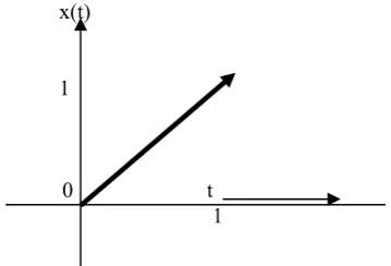
Ramp Function r(t) states that the signal will start from time zero and instantly will take a slant shape and depending upon given time characteristics (i.e. either positive or negative, here positive) the signal will follow the straight slant path either towards right or left, here towards right. Thus, the ramp function r(t) is a type of elementary function which exists only for positive side and is zero for negative. The continuous time ramp function is denoted by r(t) and may be represented in equation form as be shown below. This equation is pictorially depicted as in figure 1[1], [2], [3]. In other words, the ramp function r(t) is that type of elementary function which exists only in positive side and is zero for negative side.
The continuous-time ramp function is denoted by r(t) and is expressed mathematically as –
r(t) = t, if t >= 0
0, otherwise (that is, for t < 0)
To understand this, let us understand the example of r(t). It can be depicted as –
let x(t) = r(t)
Proposed Concept of Signals
for Ramp Functions
x(t) 1
[image:2.595.70.250.63.185.2]0 t 1
Figure 1. Ramp function r(t) based on existing theory. Now if someone asks to depict the signal r(t) – 2r(t-2) + 4r(t-3) – 2r(t-5) then it creates ambiguities that is when complex equations are given to draw then it becomes complex to draw.
Here, I will try to present the logic regarding elementary signal r(t). My theory[4] says if we are provided with a set of
ramp functions signals in the form of equations and are asked to depict on paper then it will be very easy to depict the diagram if we use the concept of angles. Here, for ramp
signals remember to have 45 degree angle shift concept. How? Solution – first we learn how to draw r(t) for which shape is given in figure 1 and then we will learn how to draw r(-t), -r(t) and lastly –r(-t).
IV. ANGLES IN RAMP FUNCTION[4]
Ramp signals 450 Concept. How is it used, we will see in the coming paragraphs.
Drawing of Different Ramp Functions Using Angles[4].
A. Drawing of r(t)[4]
Figure 3 shows that there is actually one 45 degree shift in ramp function, it is explained with the help of first by taking a ramp function r(t) -
Mathematically r(t) is represented as – r(t) = 0, when t < 0
t, otherwise (that is for t > 0)
For r(t) case, r(t) can be represented in terms of angles as shown below –
r(t) = 0, when t < 0
t, 450 anticlockwise w.r.t. x axis & at t = 0
1. First assume that, in idle case when no signal is there, then signal r(t) is assumed to come on x-axis from negative infinity to origin. This condition is shown in figure 2.
r(t)
-∞
0 t
Figure 2. Sketching function r(t) using angle theory, step 1. 2. As soon as the signal r(t) comes/appears then the signal takes a 45 degree shift in anticlockwise direction with respect to x axis and takes one straight slanted line in first quadrant i.e. takes one slant straight line in between x and y axis. r(t)
[image:2.595.361.515.63.149.2]
1 450 0 t
Figure 3. Sketching function r(t) using angle theory, step 2. 3. Lastly, this slant straight line extends upto infinity at an angle of 450 in first quadrant. This is shown in figure 3.
Hence, it states that the signal will start from time zero and takes a slant shape in first quadrant with an angle of 450 and depending upon given time characteristics (i.e. either positive or negative, here positive) the signal will follow the slant 450 path at either towards in first quadrant or in second quadrant, here in first quadrant. Thus, the ramp function r(t) is that type of elementary function which exists only for first quadrant and is zero for other quadrants. Also the ramp function is discontinuous at t <= 0. This is what I call concept of 45 degree related to ramp function r(t) .
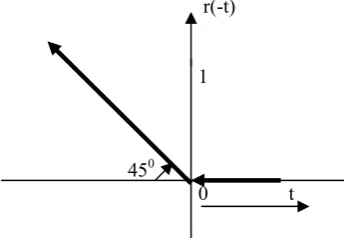
B. Drawing of r(-t )[4]
Mathematically r(-t) is represented[1], [2], [3] as – r(-t) = 0, when t < 0
t, otherwise (that is for t > 0)
For r(-t) case, r(-t) can be represented in terms of angles as shown below. Figure 4 shows that there is one 45 degree shift, it is represented as below–
r(-t) = 0, when t < 0
t, 450 clockwise w.r.t –x axis & at t = 0
[image:2.595.373.531.230.325.2]x(t)= r(-t)
1
0 t
[image:3.595.81.246.52.185.2]
Figure 4. Ramp function r(-t) based on existing theory. For r(-t) case
1. First assume that, in idle case when no signal is there then the depiction line comes from positive infinity to origin. This condition is shown in figure 5.
r(t)
[image:3.595.314.531.95.237.2]
-∞ 0 t
Figure 5. Sketching function r(-t) using angle theory, step 1. 2. As soon as the signal r(-t) comes/appears then the signal takes a 450 degree shift in clockwise direction with respect to –x axis and takes one slant straight line in between -x and y axis. This situation is shown in figure 6.
r(-t)
1
450
0 t
Figure 6. Sketching function r(-t) using angle theory, step 2. 3. This slant straight line should extend upto infinity at an angle of 450 in second quadrant. This is shown in figure 6.
Thus r(-t) signal takes one 450 shift in second quadrant in clockwise direction with respect to –x axis and extends upto infinity.
C. Drawing of -r(t)[4]
Mathematically -r(t) is represented as – -r(t) = 0, when t < 0
-t, otherwise (that is for t > 0)
For -r(t) case, -r(t) can be represented in terms of angles as shown below. Figure 7 shows that there is one 45 degree shift, it is represented as below–
-r(t) = 0, when t < 0
-t, 450 clockwise w.r.t x axis & at t = 0
x(t)= -r(t)
0 t
[image:3.595.110.261.266.373.2]
Figure 7. Ramp Function –r(t) based on existing theory. For -r(t) case
1. First assume that, in idle case when no signal is there then the depiction line comes from negative infinity to origin. This condition is shown in figure 8.
r(t)
[image:3.595.319.524.333.419.2]
-∞ 0 t
Figure 8. Sketching function -r(t) using angle theory, step 1. 2. As soon as the signal -r(t) comes/appears then the signal takes a 450 degree shift in clockwise direction with respect to x axis and takes one slant straight line in between x and -y axis. This situation is shown in figure 9.
r(-t)
-∞ 450 t
Figure 9. Sketching function -r(t) using angle theory, step 2. 3. This slant straight line extends upto infinity at an angle of 450 in fourth quadrant. This is shown in figure 9.
Thus -r(t) signal takes one 450 degrees shift in fourth quadrant in clockwise direction with respect to x axis and extends upto infinity.
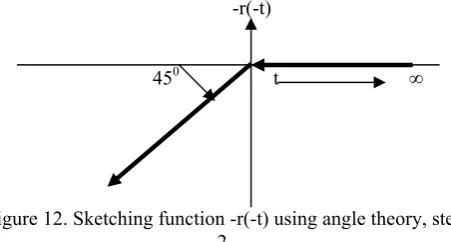
D. Drawing of –r(-t)[4]
Mathematically -r(-t) is represented as – -r(-t) = 0, when t > 0
[image:3.595.86.259.463.582.2] [image:3.595.310.537.500.604.2]For -r(-t) case, -r(-t) can be represented in terms of angles as shown below. Figure 10 shows that there is one 45 degree shift, it is represented as below–
-r(-t) = 0, when t < 0
-t, 450 anticlockwise w.r.t -x axis & at t = 0
x(t)= -r(-t)
0 t
[image:4.595.54.265.88.233.2]
Figure 10. Ramp function –r(-t) based on existing theory. For -r(-t) case
1. First assume that, in idle case when no signal is there then the depiction line comes from positive infinity to origin. This condition is shown in figure 11.
-r(-t)
[image:4.595.340.484.412.490.2]
0 t
Figure 11. Sketching function -r(-t) using angle theory, step 1.
2. As soon as the signal -r(-t) comes/appears then the signal takes a 450 degree shift in anticlockwise direction with respect to -x axis and takes one slant straight line in between -x and -y axis. This situation is shown in figure 12.
-r(-t)
[image:4.595.56.282.509.630.2]
450 t ∞
Figure 12. Sketching function -r(-t) using angle theory, step 2.
3. This slant straight line extends upto infinity at an angle of 450 in third quadrant. This is shown in figure 12.
Thus -r(-t) signal takes one 450 degrees shift in third quadrant in anticlockwise direction with respect to -x axis and extends upto infinity.
Special note - How 450 has been achieved, this is a
tedious job. Understanding of different types of ramp functions such as r(t), -r(t) etc. is of course easy but for understanding and exploring signals such as 2r(t), 3r(t), 4r(t) etc. we require a lot of exercise.
1. Let us dig out the r(t) function –
If function r(t) is represented in tabular form as shown below then we can easily see that it is very easy to get the concept of 450 angle in r(t) functions.
Table 1. Value of r(t) for varying values of time t.
t 1 2 4 5
r(t) 1 2 4 5
It is observed that function r(t) takes same value as the time takes. Thus if this table is depicted on a graph paper then it is easily understood that the angle made by these ordinates comes equal to 450. How it has been calculated - it has been calculated with the help of trigonometry by using tan function. As we know that tan always gives angle 450 if its numerator and denominator are having same values and we observe from the table that x-axis is marked as time t and y-axis is marked as function r(t) and both have same values. Hence, if tan a = x/y = r(t) / t = 1, then we get always angle 450 for function r(t). Thus, whenever r(t) is found in any of the form such as r(t), r(-t), -r(t), -r(-t), then straight way one can think of having always an angle of 450, however each will have different directions depending upon the type of function.
Consideration of 2r(t) with the help of angles and tabulation –
Roughly, as mentioned earlier, it can be shown as –
2
2r(t)
0
time
Figure 13. Function 2r(t) is normally as above. This does not give any technical idea regarding complexity of the function as this diagram has been plotted in a running hand and make sure almost all the books have given the same procedure which I think is not correct.
Let us dig out this with the help of table –
2r(t) = 2t, for t > or = to 0 0, otherwise
[image:4.595.321.463.705.733.2]Even this 2r(t) = 2t is also not defined clearly. Well, let now tabulate this function –
Table 2. Value of 2r(t) for varying values of time t.
t 1 2 4 5
2r(t)= 2t 2 4 8 10
10 8 6
4 2r(t) 2
63.440
[image:5.595.102.260.82.241.2]0 1 2 3 4 5 time t
Figure 14. Sketching function 2r(t) using angle theory.
If we observe figure 14 closely, then it can be easily visualized that this angle is not exactly 45 degree but more than the 45 degree. Then what should be the exact shape of this diagram when ramp function is 2r(t). It can be calculated with the help of trigonometry formula using tan. Here x-axis = t = 1 and y-axis = 2t. That is, angle could be taken out as inverse tan 2/1 = 63.440. Now it can be said that exact shape of the 2r(t) is one which has an angle of 63.44450. And this shape is true for further numerical equations. Thus exact shape says, if 2r(t) ramp function is given then its y and x ratios will be 2:1 i.e. 2/1 means if one uses graph paper then if for time t one goes one step or unit towards x-axis then magnitude in y-axis should be two. Now, if one measures the angle with the help of ‘D’ then he/she will find this angle equal to approximately 63 or 64 degree which is exactly equals to 63.44 degrees.
Similarly, for 3r(t) is calculated to an angle of 71.570 and likewise different r(t) functions are given as below -
4r(t) = 75.96 degrees 5r(t) = 78.69 degrees 6r(t) = 80.54 degrees 7r(t) = 81.87 degrees 8r(t) = 82.88 degrees etc.
Thus we observe that each ramp function always has an angle less than 90 degrees except infinite r(t) function which has 90 degrees exactly.
Now problem comes, most of the books those that have given numerical equations on this topic have roughly drawn the figures, which on the basis of the above analysis, I think are wrong. Thus to solve these equations specially ramp functions, it is necessary to use graph papers and/or ‘D’ so that exact points and angles can be measured and fitted accurately.
To eliminate this doubt, some examples can be done on graph papers so that exact solution can be obtained.
For the simplicity, here in this context I will consider only examples on r(t) function only.
V. EXAMPLES BASED ON THEORY DEVELOPED
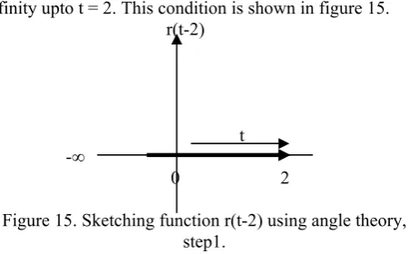
Example 1. Drawing of r(t-2) Solution –
1. First solve the time t-2 part. Time part is equated to zero i.e. t-2 = 0 or t = 2. This shows that this signal will start from t = 2 sec.
2. Now consider that, in idle case when no signal is there, then signal r(t-2) is assumed to come on x-axis from negative infinity upto t = 2. This condition is shown in figure 15. r(t-2)
t -∞
[image:5.595.314.540.197.337.2]0 2
Figure 15. Sketching function r(t-2) using angle theory, step1.
3. As soon as the signal r(t-2) comes/appears at t = 2, then the signal takes a 45 degree shift in anticlockwise direction with respect to x axis and takes one straight slanted line in first quadrant i.e. takes one slant straight line in between x and y axis.
r(t-2)
450 0 2 t
Figure 16. Sketching function r(t-2) using angle theory, step2.
4. Lastly, this slant straight line extends upto infinity at an angle of 450 in first quadrant. This is shown in figure 16.
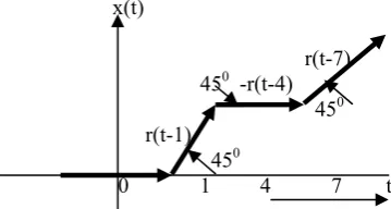
Example 2. Drawing of x(t) = r(t-7) - r(t-4) + r(t-1) Solution –
1. Before solving this, first look which part of time digit is least. In this, time t-1 part has least digit. Now, time part is equated to zero i.e. t-1 = 0 or t = 1. This shows that this signal will start from t = 1 sec.
[image:5.595.343.526.410.533.2]x(t)
-∞
[image:6.595.70.280.65.149.2]0 1 t
Figure 17. Sketching function x(t) using angle theory, step1. 3. As soon as the signal r(t-1) comes/appears at t = 1, then the signal takes a 45 degree shift in anticlockwise direction with respect to x axis and takes one straight slanted line in first quadrant i.e. takes one slant straight line in between x and y axis.
x(t)
1
[image:6.595.306.486.101.197.2]r(t-1) 450 0 1 4 t
Figure 18. Sketching function x(t) using angle theory, step2. 4. Now, take next least digit time part which is -r(t-4). Observe from discussion in this paper, this part -r(t-4) remains on r(t-1) i.e. now we consider that -r(t-4) is coming from the same path as followed by r(t-1). Now, take a shift of 450 in clockwise direction at t=4 i.e now it becomes 00 upto t = 7 as shown in figure 19.
x(t)
-r(t-4) 450 r(t-1)
450 0 1 4 t
Figure 19. Sketching function x(t) using angle theory, step3. 5. Now, take next least digit time part i.e. last part which is r(t-7). Observe from discussion in this paper, this part r(t-7) remains on -r(t-4) i.e. now we consider that r(t-7) is coming from the same path as followed by -r(t-4). Now, take a shift of 450 in clockwise direction at t = 7 i.e now it becomes 450 as shown in figure m. And lastly, it extends upto infinity.
Similarly, other complicated examples can be considered based on 2r(t), 3 r(t), 4 r(t), 5 r(t) etc. but these required extra skill either graph papers or ‘D’.
Now it might be cleared that each and every ramp function is having one 450 angles hence the theory developed fits best in the numerical examples.
Likewise some other complex examples can be considered for better understanding of the theory developed.
This is what I call concept of 45 degree related to ramp function r(t). This concept plays a vital role while solving the related numerical.
x(t)
r(t-7) 450 -r(t-4)
450 r(t-1)
[image:6.595.105.282.253.370.2]450 0 1 4 7 t
Figure 20. Sketching function x(t) using angle theory, step4.
VI. CONCLUSION
When I applied this theory to the B.Tech. (Subject : Signals and Systems) students, then I found that students not only grasped this theory but also solved a number of problems based on this.
This paper is an outcome from the teaching experience where the students faced a lot of problems to understand the ramp function numerical problems. This work is an attempt to teach the students step by step construction procedure of ramp signal functions and this work has an attempt to explore the new and easy theory specially written for ramp related to the basic signal functions. No doubt the future studies will further explore my work in deep.
On the basis of this theory, some other signals could be developed that will go long to the scientists and students. As no matter is available on the internet, hence I claim that this theory is purely based on my research work/affords and has a
bright chance to explore new theory and ideas on this. .
ACKNOWLEDGMENT
I would like to thank to my B.Tech. pursuing students who posed a lot of questions in the form of doubts and inclined me to think more and more to clarify their complex doubts. What I feel in this context that it is only the students for a teacher who can make a teacher gold from silver. Hence, I acknowledge my students and again I pay special thanks to my students who made me to reach at this stage where I could produce this paper.
REFERENCE
[1] A.V. Oppenheim, A.S. Willsky with S. Hamid Nawab, Signals and Systems – by – Pearson Education, Second edition, 2002.
[2] Simon Haykin, Barry Van Veen, Signals and systems – by – John Wiley & Sons (Asia) Pte. Ltd., Second Edition, 2004 .
[3] P. Ramakrishna Rao, Signals and Systems – by – Tata McGraw Hill, First edition, 2008.
[image:6.595.103.258.476.584.2]