Feature Selection as Causal Inference: Experiments with Text Classification

Feature Selection as Causal Inference:

Experiments with Text Classification

Michael J. Paul University of Colorado Boulder, CO 80309, USA

mpaul@colorado.edu

Abstract

This paper proposes a matching tech-nique for learning causal associations be-tween word features and class labels in document classification. The goal is to identify more meaningful and general-izable features than with only correla-tional approaches. Experiments with sen-timent classification show that the pro-posed method identifies interpretable word associations with sentiment and improves classification performance in a majority of cases. The proposed feature selection method is particularly effective when ap-plied to out-of-domain data.

1 Introduction

A major challenge when building classifiers for high-dimensional data like text is learning to iden-tify features that are not just correlated with the classes in the training data, but associated with classes in a meaningful way that will generalize to

new data. Methods for regularization (Hoerl and

Kennard, 1970; Chen and Rosenfeld, 2000) and

feature selection (Yang and Pedersen, 1997;

For-man,2003) are critical for obtaining good

classi-fication performance by removing or minimizing the effects of noisy features. While empirically successful, these techniques can only identify fea-tures that are correlated with classes, and these as-sociations can still be caused by factors other than the direct relationship that is assumed.

A more meaningful association is acausalone.

In the context of document classification using bag-of-words features, we ask the question, which word features “cause” documents to have the class labels that they do? For example, it might be

rea-sonable to claim that adding the wordhorribleto a

review would cause its sentiment to become

neg-ative, while this is less plausible for a word like

said. Yet, in one of our experimental datasets

of doctor reviews, saidhas a stronger correlation

with negative sentiment thanhorrible.

Inspired by methods for causal inference in other domains, we seek to learn causal asso-ciations between word features and document classes. We experiment with propensity score

matching (Rosenbaum and Rubin, 1985), a

tech-nique attempts to mimic the random assignment of subjects to treatment and control groups in a randomized controlled trial by matching subjects with a similar “propensity” to receive treatment. Translating this idea to document classification, we match documents with similar propensity to contain a word, allowing us to compare the effect a word has on the class distribution after controlling for the context in which the word appears. We pro-pose a statistical test for measuring the importance of word features on the matched training data.

We experiment with binary sentiment classifi-cation on three review corpora from different do-mains (doctors, movies, products) using propen-sity score matching to test for statistical signifi-cance of features. Compared to a chi-squared test, the propensity score matching test for feature se-lection yields superior performance in a majority of comparisons, especially for domain adaptation and for identifying top word associations. After

presenting results and analysis in Sections4–5, we

discuss the implications of our findings and make suggestions for areas of language processing that would benefit from causal learning methods.

2 Causal Inference and Confounding

A challenge in statistics and machine learning is identifying causal relationships between variables. Predictive models like classifiers typically learn only correlational relationships between variables,

and if spurious correlations are built into a model, then performance will worsen if the underlying distributions change.

A common cause of spurious correlations is

confounding. A confounding variable is a vari-able that explains the association between a depen-dent variable and independepen-dent variables. A com-monly used example is the positive correlation of ice cream sales and shark attacks, which are corre-lated because they both increase in warm weather (when more people are swimming). As far as any-one is aware, ice cream does not cause shark at-tacks; rather, both variables are explained by a confounding variable, the time of year.

There are experimental methods to reduce con-founding bias and identify causal relationships. Randomized controlled trials, in which subjects are randomly assigned to a group that receives treatment versus a control group that does not, are the gold standard for experimentation in many do-mains. However, this type of experiment is not always possible or feasible. (In text processing, we generally work with documents that have al-ready been written: the idea of assigning features to randomly selected documents to measure their effect does not make sense, so we cannot directly translate this idea.)

A variety of methods exist to attempt to in-fer causality even when direct experiments, like randomized controlled trials, cannot be conducted (Rosenbaum,2002). In this work, we propose the use of one such method, propensity score

match-ing (Rosenbaum and Rubin, 1985), for reducing

the effects of confounding when identifying im-portant features for classification. We describe this

method, and its application to text, in Section 3.

First, we discuss why causal methods may be im-portant for document classification, and describe previous work in this space.

2.1 Causality in Document Classification

We now discuss where these ideas are relevant to document classification. Our study performs sen-timent classification in online reviews using bag-of-words (unigram) features, so we will use exam-ples that apply to this setting.

There are a number of potentially confounding

factors in document classification (Landeiro and

Culotta,2016). Consider a dataset of restaurant re-views, in which fast food restaurants have a much lower average score than other types of

restau-rants. Word features that are associated with fast

food, likedrive-thru, will be correlated with

neg-ative sentiment due to this association, even if the word itself has neutral sentiment. In this case, the type of restaurant is a confounding variable that causes spurious associations. If we had a method for learning causal associations, we would know thatdrive-thruitself does not affect sentiment.

What does it mean for a word to have a causal relationship with a document class? It is difficult to give a natural explanation for a bag-of-words model that ignores pragmatics and discourse, but here is an attempt. Suppose you are someone who understands bag-of-words representations of doc-uments, and you are given a bag of words corre-sponding to a restaurant review. Suppose

some-one adds the wordterribleto the bag. If you

pre-viously recognized the sentiment to be neutral or even positive, it is possible that the addition of this new word would cause the sentiment to change to negative. On the other hand, it is hard to imagine a

set of words to which adding the worddrive-thru

would change the sentiment in any direction. In this example, we would say that the word

terrible “caused” the sentiment to change, while

drive-thru did not. While most real documents will not have a clean interpretation of a word “causing” a change in sentiment, this may still serve as a useful conceptual model for identify-ing features that are meanidentify-ingfully associated with class labels.

2.2 Previous Work

Recent studies have used text data, especially

so-cial media, to make causal claims (Cheng et al.,

2015; Reis and Culotta, 2015; Pavalanathan and Eisenstein, 2016). The technique we use in this work, propensity score matching, has recently

been applied to user-generated text data (Rehman

et al.,2016;De Choudhury and Kiciman,2017). For the task of document classification

specif-ically, Landeiro and Culotta (2016) experiment

with multiple methods to make classifiers robust to confounding variables such as gender in social media and genre in movie reviews. This work re-quires confounding variables to be identified and included explicitly, whereas our proposed method requires only the features used for classification.

Causal methods have previously been applied

to feature selection (Guyon et al., 2007;Cawley,

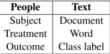
match-People Text

Subject Document

Treatment Word

Outcome Class label

Table 1: A mapping of standard terminology of randomized controlled trials (left) to our applica-tion of these ideas to text classificaapplica-tion (right).

ing methods proposed in this work, and not for document classification.

3 Propensity Score Matching for Document Classification

Propensity score matching (PSM) (Rosenbaum

and Rubin,1985) is a technique that attempts to simulate the random assignment of treatment and control groups by matching treated subjects to un-treated subjects that were similarly likely to be in the same group. This is centered around the idea of apropensity score, whichRosenbaum and Rubin

(1983) define as the probability of being assigned

to a treatment group based on observed character-istics of the subject,P(zi|xi), typically estimated

with a logistic regression model. In other words, what is the “propensity” of a subject to obtain treatment? Subjects that did and did not receive treatment are matched based their propensity to re-ceive treatment, and we can then directly compare the outcomes of the treated and untreated groups.

In the case of document classification, we want to measure the effect of each word feature. Using the terminology above, each word is a “treatment” and each document is a “subject”. Each word has a treatment group, the documents that contain the word, and a “control” group, the documents that do not. The “outcome” is the document class label. Each subject has a propensity score for a treat-ment. In document classification, this means that each document has a propensity score for each word, which is the probability that the word would

appear in the document. For a wordw, we define

this as the probability of the word appearing given

all other words in the document:P(w|di− {w}),

wheredi is the set of words in theith document.

We estimate these probabilities by training a logis-tic regression model with word features.

Using our example from the previous section, the probability that a document contains the word

drive-thru is likely to be higher in reviews that describe fast food that those that do not.

Match-ing reviews based on their likelihood of contain-ing this word should adjust for any bias caused by the type of restaurant (fast food) as a confounding variable. This is done without having explicitly in-cluded this as a variable, since it will implicitly be learned when estimating the probability of words

associated with fast food, likedrive-thru.

3.1 Creating Matched Samples

Once propensity scores have been calculated, the next step is to match documents containing a word to documents that do not contain the word but have a similar score. There are a number of strategies

for matching, summarized byAustin(2011a). For

example, matching could be done one-to-one or one-to-many, sampling either with or without re-placement. Another approach is to group similar

scoring samples into strata (Cochran,1968).

In this work, we perform one-to-one ing without replacement using a greedy

match-ing algorithm; Gu and Rosenbaum (1993) found

no quality difference using greedy versus optimal matching. We also experiment with thresholding how similar two scores must be to match them.

Implementation Even greedy matching is ex-pensive, so we use a fast approximation. We place documents into 100 bins based on their scores

(e.g., scores between .50 and .51). For each

“treatment” document, we match it to the approx-imate closest “control” document by pointing to the treatment document’s bin and iterating over bins outward until we find the first non-empty bin, and then select a random control document from that bin. Placing documents into bins is related to

stratification approaches (Rosenbaum and Rubin,

1984), except that we use finer bins that typical

strata and we still return one-to-one pairs.

3.1.1 Comparing Groups

Since our instances are paired (after one-to-one

matching), we can use McNemar’s test (

McNe-mar, 1947), which tests if there is a significant

change in the distribution of a variable in response to a change in the other. The test statistic is:

χ2 ₌ (T N −CP)2

T N+CP (1)

where T N is the number of treatment instances

with a negative outcome (in our case, the num-ber of documents containing the target word with

a negative sentiment label) andCP is the number

# documents # tokens # word types Doctors 20,000 432,636 2,422

Movies 50,000 9,420,645 3,124 Products 100,000 7,416,381 2,343

Table 2: Corpus summary.

number of documents that do not contain the word with a positive sentiment label).

This test statistic has a chi-squared distribution with 1 degree of freedom. This test is related to a traditional chi-squared test used for feature se-lection (which we compare to experimentally in

Section4), except that it assumes paired data with

a “before” and “after” measurement. In our case, we do not have two outcome measurements for the same subject, but we have two subjects that have been matched in a way that approximates this.

We perform this test for every feature (every word in the vocabulary). The goal of the test is to measure there is a significant difference in the class distribution (positive versus negative, in the case of sentiment) in documents that do and do not contain the word (the “after” and “before” con-ditions, respectively, when considering words as treatments).

4 Experiments with Feature Selection

To evaluate the ability of propensity score match-ing to identify meanmatch-ingful word features, we use it

for feature selection (Yang and Pedersen,1997) in

sentiment classification (Pang and Lee,2004).

4.1 Datasets

We used datasets of reviews from three domains:

• Doctors: Doctor reviews from RateMDs.com (Wallace et al., 2014). Doctors are rated on a scale from 1–5 along four different dimensions (knowledgeability, staff, helpfulness, punctual-ity). We averaged the four ratings for each re-view and labeled a rere-view positive if the average

rating was≥4and negative if≤2.

• Movies: Movie reviews from IMDB (Maas et al.,2011). Movies are rated on a scale from

1–10. Reviews rated ≥ 7 are labeled positive

and reviews rated≤4are labeled negative.

• Products: Product reviews from Amazon ( Jin-dal and Liu,2008). Products are rated on a scale

from 1–5, with reviews rated≥4labeled

posi-tive and reviews rated≤2labeled negative.

All datasets were sampled to have an equal class balance. We used unigram word features. For

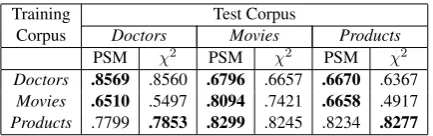
ef-Training Test Corpus

Corpus Doctors Movies Products

PSM χ2 _{PSM χ}2 _{PSM χ}2

Doctors .8569 .8560 .6796 .6657 .6670 .6367

Movies .6510 .5497 .8094 .7421 .6658 .4917

Products .7799 .7853 .8299 .8245 .8234 .8277

Table 3: Area under the feature selection curve

(see Figure 1) using F1-score as the evaluation

metric. All differences between corresponding

PSM and χ2 _{results are statistically significant}

withp0.01except for (Doctors,Doctors).

ficiency reasons (a limitation that is discussed in

Section7), we pruned the long tail of features,

re-moving words appearing in less than 0.5% of each corpus. The sizes of the processed corpora and

their vocabularies are summarized in Table2.

4.2 Experimental Details

For each corpus, we randomly selected 50% for training, 25% for development, and 25% for test-ing. The training set is used for training classifiers as well as calculating all feature selection metrics. We used the development set to measure clas-sification performance for different hyperparame-ter values. Our propensity score matching method has two hyperparameters. First, when building lo-gistic regression models to estimate the propensity

scores, we adjusted the`2regularization strength.

Second, when matching documents, we required the difference between scores to be less than

τ×SDto count as a match, whereSDis the

stan-dard deviation of the propensity scores. We

per-formed a grid search over different values ofτ and

different regularization strengths, described more

in our analysis in Section 5.2, and used the best

combination of hyperparameters for each dataset. We used logistic regression classifiers for sen-timent classification. While we experimented

with`2 regularization for constructing propensity

scores, we used no regularization for the sentiment classifiers. Since regularization and feature selec-tion are both used to avoid overfitting, we did not want to conflate the effects of the two, so by us-ing unregularized classifiers we can directly assess the efficacy of our feature selection methods on held-out data. All models were implemented with

scikit-learn(Pedregosa et al.,2011).

Baseline We compare propensity score

match-ing with McNemar’s test(PSM)to a standard

0.0 0.2 0.4 0.6 0.8 1.0

Percentage of feature set

0.75 0.80 0.85 0.90

F1 score

Doctors

PSM χ2

0.0 0.2 0.4 0.6 0.8 1.0

Percentage of feature set

0.60 0.65 0.70 0.75 0.80 0.85 0.90

F1 score

Movies

PSM χ2

0.0 0.2 0.4 0.6 0.8 1.0

Percentage of feature set

0.60 0.65 0.70 0.75 0.80 0.85

F1 score

Products

PSM χ2

Figure 1: F1 scores when using a varying numbers of features ranked by two feature selection tests.

most common statistical tests for features in

doc-ument classification (Manning et al.,2008). Since

both tests follow a chi-squared distribution, and since McNemar’s test is loosely like a chi-squared test for paired data, we believe this baseline offers the most direct comparison.

4.3 Results

We calculated the F1 scores of the sentiment clas-sifiers when using different numbers of features ranked by significance. For example, when train-ing a classifier with 1% of the feature set, this is the most significant 1% (with the lowest p-values). Results for varying feature set sizes on the three

test datasets are shown in Figure1.

To summarize the curves with a concise metric, we calculated the area under these curves (AUC). AUC scores for each dataset can be found along

the diagonal of Table3. We find that PSM gives

higher AUC scores than χ2 _{in two out of three}

datasets, though one is not statistically significant based on a paired t-test of the F1 scores.

PSM gives a large improvement overχ2 _{on the}

Moviescorpus, though the feature selection curve is unusual in that it rises gradually and peaks much

later thanχ2_{. This appears to be because the}

high-est ranking words with PSM have mostly positive sentiment. There is a worse balance of class

asso-ciations in the top features with PSM thanχ2_{, so}

the classifier has a harder time discriminating with few features. However, PSM eventually achieves

a higher score than the peak fromχ2 _{and the}

per-formance does not drop as quickly after peaking. In the next two subsections, we examine addi-tional settings in which PSM offers larger

advan-tages over theχ2_baseline.

4.3.1 Generalizability

A motivation for learning features with causal as-sociations with document classes is to learn robust

Doctors Movies Products

PSM χ2 _{PSM χ}2 _{PSM χ}2

great told great worst excellent waste

caring great excellent bad wonderful money

rude rude wonderful and great great

best best best great waste worst

excellent said love waste bad best

Table 4: The highest scoring words from the two feature selection methods.

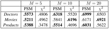
M= 5 M= 10 M= 20

PSM χ2 _{PSM χ}2 _{PSM χ}2

Doctors .5573 .4806 .6318 .5520 .6999 .6503

Movies .5211 .4962 .5841 .6196 .6171 .6921

Products .5388 .3478 .5514 .4696 .6031 .5622

Table 5: Area under the feature selection curve

when using only a small number of features,M.

features that can generalize to changes in the data distribution. To test this, we evaluated each of the three classifiers on the other two datasets (for

ex-ample, testing the classifier trained onDoctorson

theProductsdataset). The AUC scores for all pairs

of datasets are shown in Table3.

On average, PSM improves the AUC over χ2

by an average of.021when testing on the same

domain as training, while the improvement

in-creases to an average of.053when testing on

out-of-domain data. In thus seems that PSM may be particularly effective at identifying features that can be applied across domains.

4.3.2 Top Features

Having measured performance across the entire feature set, we now focus on only the most highly associated features. The top features are important because these can give insights into the classifica-tion task, revealing which features are most asso-ciated with the target classes. Having top features that are meaningful and interpretable will lead to

iden-tifying meaningful features can itself be the goal of a study (Eisenstein et al.,2011b).

We experimented with a small number of

fea-turesM ∈ {5,10,20}. Under the assumption that

optimal hyperparameters may be different when using such a small number of features, we retuned the PSM parameters again for the experiments in

this subsection, usingM=10.

Table 4 shows the five words with the lowest

p-values with both methods. At a glance, the top words from PSM seem to have strong sentiment

associations; for example, excellent is a top five

feature in all three datasets using PSM, and none

of the datasets usingχ2_{. Words without obvious}

sentiment associations seem to appear more often

in the topχ2_{features, likeand.}

To quantify if there is a difference in quality, we again calculated the area under the feature se-lection F1 curves, where the number of features

ranged from 1 toM. Results are shown in Table5.

ForM of10and20, PSM does worse onMovies,

which is not surprising based on our finding above that the top features in this dataset are not bal-anced across the two labels, so PSM does worse for smaller numbers of features. For the other two

datasets, PSM substantially outperformsχ2_{. PSM}

appears to be an effective method for identifying strong feature associations.

5 Empirical Analysis

We now perform additional analyses to gain a deeper understanding of the behavior of propen-sity score matching applied to feature selection.

5.1 An Example

To better understand what happens during

match-ing, we examined the word said on the Doctors

corpus. This word does not have an obvious sen-timent association, but is the fifth-highest scoring

word with χ2_{. It is still highly ranked when}

us-ing propensity score matchus-ing, but this approach reduces its rank to ten.

Upon closer inspection, we find that reviews tend to use this word when discussing logistical issues, like interactions with office staff. These issues seem to be discussed primarily in a

nega-tive context, givingsaida strong association with

negative sentiment. If, however, reviews that dis-cussed these logistical issues were matched, then within these matched reviews, those containing

saidare probably not more negative than those that

0.01 0.1 1.0 100.0 109

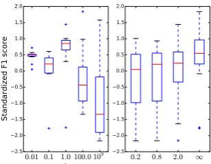
λ

2.5 2.0 1.5 1.0 0.5 0.0 0.5 1.0 1.5 2.0

Standardized F1 score

0.2 0.8 2.0 ∞

τ

2.5 2.0 1.5 1.0 0.5 0.0 0.5 1.0 1.5 2.0

Figure 2: The distribution of the area under the feature selection curve scores when using different hyperparameter settings (propensity inverse

regu-larization strengthλand matching thresholdτ).

0.01 0.1 1.0 100.0 109

λ

2.5 2.0 1.5 1.0 0.5 0.0 0.5 1.0 1.5 2.0

Standardized F1 score

τ=∞

0.2 0.8 2.0 ∞

τ

2.5 2.0 1.5 1.0 0.5 0.0 0.5 1.0 1.5

2.0 λ=1.0

Figure 3: The distribution of scores when using different hyperparameter settings, restricted to the best performing setting for each independent

pa-rameter as shown in Figure2(varyingλwith the

optimalτ, and varyingτ with the optimalλ).

do not. With propensity score matching, docu-ments are matched based on how likely they are

to contain the wordsaid, which is meant to

con-trol for the negative context that this word has a tendency (or propensity) to appear in.

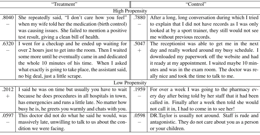
Table 6 shows example reviews that do (the

“treatment” group) and do not (the “control”

group) contain said. We see that the higher

propensity reviews do tend to discuss issues like receptionists and records, and controlling for this context may explain why this method produced a lower ranking for this word.

5.2 Hyperparameter Settings

We investigate the effect of different hyperparam-eter settings. To do this, we first standardized the results across the three development datasets by converting them to z-scores so that they can be directly compared. The distribution of scores (specifically, the area under the F1 curve scores

“Treatment” “Control” High Propensity

.8040

− She repeatedly said, “I don’t care how you feel”when my wife told her the medication (birth control) was causing issues. She failed to mention a positive test result, giving a clean bill of health.

.7880

− After a long, long conversation during which I triedto explain that I did not have records as I was only looked at by a sport trainer, they still would not see me without previous records.

.6320

− I went for a checkup and he ended up waiting forover 2 hours just to get into the room. Then I waited some more until he eventually came in and dedicated the whole 10 minutes of his time. When I asked what exactly is going to take place, the assistant said, no big deal, just a little scrape.

.5047

+ The receptionist was able to get me in the nextday and really worked around my busy schedule. I downloaded my paperwork off the website and had it ready at my appointment. I waited maybe 10 min-utes and was in the exam room. The doctor was re-ally nice and took the time to talk to me.

Low Propensity .2012

+ I said he was on time but usually you have to waitbecause he does procedures in all hospitals in town, has emergencies and runs a little late. No matter how busy he is, he greets you warmly and chats with you.

.1959

− For over a week I was going to the pharmacy ev-ery day after being told by her staff that it had been called in. Finally after a week then told she would not call it in, I had to come in to see her!

.0597

− This doctor did not do what he said he would, wasmassively late, unwilling to talk to us about the con-dition we were facing.

.0598

− DR.Taylor is usually not around. Staff is rude andantagonistic. They do not care about you as a person or your children.

Table 6: Examples of reviews that were matched based on the wordsaid. Reviews on the left contain

the wordsaidwhile those on the right do not. Each row corresponds to a pair of matched documents

(edited for length). The propensity score and sentiment label (+or−) is shown for each document.

Regularization When training the logistic re-gression model to create propensity scores, we experimented with the following values of

the inverse regularization parameter: λ ∈

{0.01,0.1,1.0,100.0,109_{}, where λ=10}9 _is

es-sentially no regularization other than to keep the optimal parameter values finite. We make two

ob-servations. First, high λ values (less

regulariza-tion) generally result in worse scores. Second,

smallλvalues lead to more consistent results, with

less variance in the score distribution. Based on

these results, we recommend a value of λ=1.0

based on its high median score, competitive maxi-mum score, and low variance.

Matching We required that the scores of two

documents were within τ×SD of each other,

and experimented with the following thresholds: τ ∈ {0.2,0.8,2.0,∞}.Austin(2011b) found that

τ=0.2 was optimal for continuous features and

τ=0.8was optimal for binary features. Based on

these guidelines,0.8would be appropriate for our

scenario, but we also compared to a larger

thresh-old (2.0) and no threshold (∞). We find that scores

consistently increase asτ increases.

Coupling Looking at the two hyperparameters independently does not tell the whole story, due to interactions between the two. In particular, we

ob-serve that lower thresholds (lower τ) work better

when using heavier regularization (lower λ), and

vice versa. It turns out that it is ill-advised to use

τ=∞, as Figure2would suggest, when using our

recommendation of λ=1.0. Figure 3 shows the

λdistribution when set toτ=∞and theτ

distri-bution when set toλ=1.0. This shows that when

λ=1.0, scores are much worse whenτ=∞. When

τ=∞, scores are better with higherλvalues.

The best combinations of hyperparameters are

(λ= 100.0, τ =∞)and(λ= 1.0, τ = 2.0).

Be-tween these, we recommend(λ = 1.0, τ = 2.0)

due to its higher median and lower variance.

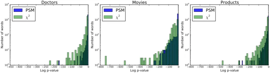
5.3 P-Values

Lastly, we examine the p-values produced by Mc-Nemar’s test on propensity score matched data compared to the standard chi-squared test.

Fig-ure 4 shows the distribution of the log of the

p-values from both methods, using the same

hyper-parameters as in Section4.3. We find thatχ2_tends

to assign lower p-values, with more extreme val-ues. This suggests that propensity score matching yields more conservative estimates of the statisti-cal significance of features.

6 Related Work

450 400 350 300 250 200 150 100 50 0

Log p-value

100 101 102 103 104

Number of words

Doctors PSM

χ2

800 700 600 500 400 300 200 100 0

Log p-value

100 101 102 103 104

Number of words

Movies PSM

χ2

800 700 600 500 400 300 200 100 0

Log p-value

100 101 102 103 104

Number of words

Products PSM

χ2

Figure 4: Distribution of p-values of features from the two methods of testing. Counts are on a log scale.

Matching There have been instances of using matching techniques to improve text training data.

Tan et al. (2014) built models to estimate the number of retweets of Twitter messages and ad-dressed confounding factors by matching tweets of the same author and topic (based on posting

the same link). Zhang et al. (2016) built

classi-fiers to predict media coverage of journal articles used matching sampling to select negative training examples, choosing articles from the same jour-nal issue. While motivated differently, contrastive

estimation (Smith and Eisner, 2005) is also

re-lated to matching. In contrastive estimation, nega-tive training examples are synthesized by perturb-ing positive instances. This strategy essentially matches instances that have the same semantics but different syntax.

Annotation Perhaps the work that most closely gets at the concept of causality in document classi-fication is work that asks for annotators to identify which features are important. There are branches of active learning which ask annotators to label not only documents, but to label features for

impor-tances or relevance (Raghavan et al.,2006;Druck

et al.,2009). Work on annotator rationales (Zaidan et al., 2007; Zaidan and Eisner, 2008) seeks to

modelwhy annotators labeled a document a

cer-tain way—in other words, what “caused” the doc-ument to have its label? These ideas could poten-tially be integrated with causal inference methods for document classification.

7 Future Work

Efficiency is a drawback of the current work. The standard way of defining propensity scores with logistic regression models is not designed to scale to the large number of variables used in text clas-sification. Our proposed method is slow because it requires training a logistic regression model for

every word in the vocabulary. Perhaps documents could instead be matched based on another met-ric, like cosine similarity. This would match docu-ments with similar context, which is what the PSM method appears to be doing based on our analysis. We emphasize that the results of the PSM sta-tistical analysis could be used in ways other than using it to select features ahead of training, which is less common today than doing feature selection directly through the training process, for

exam-ple with sparse regularization (Tibshirani, 1994;

Eisenstein et al., 2011a; Yogatama and Smith,

2014). One way to integrate PSM with

regular-ization would be to use each feature’s test statistic to weight its regularization penalty, discouraging features with high p-values from having large co-efficients in a classifier.

In general, we believe this work shows the util-ity of controlling for the context in which features appear in documents when learning associations between features and classes, which has not been widely considered in text processing. Prior work that used matching and related techniques for text classification was generally motivated by specific factors that needed to be controlled for, but our study found that a general-purpose matching ap-proach can also lead to better feature discovery. We want this work to be seen not necessarily as a specific prescription for one method of feature se-lection, but as a general framework for improving learning of text categories.

8 Conclusion

re-liably learn if a feature has a significant, causal effect on document classes. While the concept of causality does not apply to document classification as naturally as in other tasks, the methods used for causal inference may still lead to more inter-pretable and generalizable features. This was evi-denced by our experiments with feature selection using corpora from three domains, in which our proposed approach resulted in better performance than a comparable baseline in a majority of cases, particularly when testing on out-of-domain data. In future work, we hope to consider other metrics for matching to improve the efficiency, and to con-sider other ways of integrating the proposed fea-ture test into training methods for text classifiers.

References

C.F. Aliferis, A. Statnikov, I. Tsamardinos, S. Mani, and X.D. Koutsoukos. 2010. Local causal and markov blanket induction for causal discovery and feature selection for classification. Journal of Ma-chine Learning Research11:171–234.

P.C. Austin. 2011a. An introduction to propensity score methods for reducing the effects of confound-ing in observational studies.Multivariate Behav Res

46(3):399–424.

P.C. Austin. 2011b. Optimal caliper widths for propensity-score matching when estimating differ-ences in means and differdiffer-ences in proportions in ob-servational studies. Pharm Stat10(2):150–161. G.C. Cawley. 2008. Causal & non-causal feature

se-lection for ridge regression. InProceedings of the Workshop on the Causation and Prediction Chal-lenge at WCCI 2008.

S.F. Chen and R. Rosenfeld. 2000. A survey of smoothing techniques for maximum entropy mod-els. IEEE Transactions on Speech and Audio Pro-cessing8(1):37–50.

J. Cheng, C. Danescu-Niculescu-Mizil, and J. Leskovec. 2015. Antisocial behavior in on-line discussion communities. In International Conference on Web and Social Media (ICWSM). W.G. Cochran. 1968. The effectiveness of adjustment

by subclassification in removing bias in observa-tional studies. Biometrics24:295–313.

M. De Choudhury and E. Kiciman. 2017. The lan-guage of social support in social media and its effect on suicidal ideation risk. In International Confer-ence on Web and Social Media (ICWSM).

G. Druck, B. Settles, and A. McCallum. 2009. Ac-tive learning by labeling features. InConference on Empirical Methods in Natural Language Processing (EMNLP).

J. Eisenstein, A. Ahmed, and E.P. Xing. 2011a. Sparse additive generative models of text. InInternational Conference on Machine Learning (ICML).

J. Eisenstein, N.A. Smith, and E.P. Xing. 2011b. Dis-covering sociolinguistic associations with structured sparsity. InProceedings of the Association for Com-putational Linguistics (ACL).

G. Forman. 2003. An extensive empirical study of fea-ture selection metrics for text classification.Journal of Machine Learning Research3:1289–1305. X.S. Gu and P.R. Rosenbaum. 1993. Comparison

of multivariate matching methods: Structures, dis-tances, and algorithms. Journal of Computational and Graphical Statistics2:405–420.

I. Guyon, C. Aliferis, and A. Elisseeff. 2007. Causal feature selection. In H. Liu and H. Motoda, editors,

Computational Methods of Feature Selection, Chap-man and Hall/CRC Press.

A.E. Hoerl and R.W. Kennard. 1970. Ridge regres-sion: Biased estimation for nonorthogonal prob-lems. Technometrics12:55–67.

N. Jindal and B. Liu. 2008. Opinion spam and analy-sis. InInternational Conference on Web Search and Data Mining (WSDM).

V. Landeiro and A. Culotta. 2016. Robust text classifi-cation in the presence of confounding bias. InAAAI. A.L. Maas, R.E. Daly, P.T. Pham, D. Huang, A.Y. Ng, and C. Potts. 2011. Learning word vectors for senti-ment analysis. InAnnual Meeting of the Association for Computational Linguistics (ACL).

C.D. Manning, P. Raghavan, and H. Sch¨utze. 2008.

Introduction to Information Retrieval. Cambridge University Press.

Q. McNemar. 1947. Note on the sampling error of the difference between correlated proportions or per-centages. Psychometrika12(2):153–157.

B. Pang and L. Lee. 2004. A sentimental education: Sentiment analysis using subjectivity summarization based on minimum cuts. InProceedings of the 42nd Annual Meeting on Association for Computational Linguistics (ACL).

M.J. Paul. 2016. Interpretable machine learning: lessons from topic modeling. InCHI Workshop on Human-Centered Machine Learning.

U. Pavalanathan and J. Eisenstein. 2016. Emoticons vs. emojis on Twitter: A causal inference approach. In

AAAI Spring Symposium on Observational Studies through Social Media and Other Human-Generated Content.

E. Duchesnay. 2011. Scikit-learn: Machine learning in Python. Journal of Machine Learning Research

12:2825–2830.

H. Raghavan, O. Madani, and R. Jones. 2006. Active learning with feedback on features and instances. J. Mach. Learn. Res.7:1655–1686.

N.A. Rehman, J. Liu, and R. Chunara. 2016. Using propensity score matching to understand the rela-tionship between online health information sources and vaccination sentiment. InAAAI Spring Sympo-sium on Observational Studies through Social Me-dia and Other Human-Generated Content.

V.L.D. Reis and A. Culotta. 2015. Using matched sam-ples to estimate the effects of exercise on mental health from Twitter. InAAAI.

P.R. Rosenbaum. 2002. Observational Studies. Springer-Verlag.

P.R. Rosenbaum and D.B. Rubin. 1983. The central role of the propensity score in observational studies for causal effects. Biometrika70:41–55.

P.R. Rosenbaum and D.B. Rubin. 1984. Reducing bias in observational studies using subclassification on the propensity score. Journal of the American Sta-tistical Association79:516–524.

P.R. Rosenbaum and D.B. Rubin. 1985. Constructing a control group using multivariate matched sampling methods that incorporate the propensity score. The American Statistician39:33–38.

N.A. Smith and J. Eisner. 2005. Contrastive estima-tion: Training log-linear models on unlabeled data. InProceedings of the Association for Computational Linguistics (ACL).

C. Tan, L. Lee, and B. Pang. 2014. The effect of word-ing on message propagation: Topic- and author-controlled natural experiments on Twitter. In An-nual Meeting of the Association for Computational Linguistics (ACL).

R. Tibshirani. 1994. Regression shrinkage and selec-tion via the lasso. Journal of the Royal Statistical Society, Series B58:267–288.

B.C. Wallace, M.J. Paul, U. Sarkar, T.A. Trikalinos, and M. Dredze. 2014. A large-scale quantitative analysis of latent factors and sentiment in online doctor reviews. Journal of the American Medical Informatics Association21(6):1098–1103.

Y. Yang and J.O. Pedersen. 1997. A comparative study on feature selection in text categorization. In Pro-ceedings of the Fourteenth International Conference on Machine Learning (ICML).

D. Yogatama and N.A. Smith. 2014. Linguistic struc-tured sparsity in text categorization. In Annual Meeting of the Association for Computational Lin-guistics (ACL).

O.F. Zaidan and J. Eisner. 2008. Modeling annotators: A generative approach to learning from annotator ra-tionales. InProceedings of EMNLP 2008. pages 31– 40.

O.F. Zaidan, J. Eisner, and C. Piatko. 2007. Using “an-notator rationales” to improve machine learning for text categorization. InNAACL HLT 2007; Proceed-ings of the Main Conference. pages 260–267. Y. Zhang, E. Willis, M.J. Paul, N. Elhadad, and B.C.