Abstract—The present paper describes the structure and the design aspects of a robust PID controller for higher-order systems. A design scheme that combines deadbeat response, robust control, and model reduction techniques to enhance the performances and robustness of PID controller is presented. Unlike conventional deadbeat controllers, the tuning parameters are reduced to one cascade gain which yields a practical tuning method. The design scheme is illustrated on a pitch-axis autopilot design of an Unmanned Aerial Vehicle (UAV). Computer simulations show that the proposed method improves time-domain response performances and exhibits stronger robustness property to conquer system uncertainties.
Index Terms— deadbeat controller, higher-order systems, robust control, UAV flight control system
I. INTRODUCTION
HE integration of an autopilot in the control loop of an UAV airframe provides complete set of avionics which enable the UAV to autonomously complete its mission. This electronic system is generally designed to provide intelligent and autonomous flight Navigation and Control (N&C) system to conventional airframes (stable fixed wing with aileron-elevator-rudder control surfaces and engine throttle control) for autonomous navigation between predefined waypoints. Most of modern autopilots incorporate control law algorithms to meet the demanding requirements of flight maneuvers with high performance and to successfully accomplish the mission of autonomous flight.
In recent years, considerable research into the design of algorithms for UAV autopilots using modern control theory has been completed. A large number of control algorithms have been developed for onboard N&C systems. Most of these systems include some nonlinear terms [1-3], evolutionary algorithms [4-8], or optimization techniques [9]. Despite their success, only a small number of implementations of these systems have been reported and it appears that there is not much enthusiasm to use them due to their complexity, nonlinear nature, and computation cost.
Manuscript received July 26, 2011, revised August 16, 2011. This work was supported in part by the Deanship of Scientific Research under grant T95/429 and the Aeronautical Engineering Department KAU.
B. Kada is with Department of Aeronautical Engineering, Faculty of Engineering, King Abdul-Aziz University, PO Box 80204, Jeddah 21589, KSA (corresponding author phone: 2-640-2000 Ext. 68729; fax: 966-2-695-2944; e-mail: bkada@ kau.edu.sa).
Y. Ghazzawi. is with Department of Aeronautical Engineering, Faculty of Engineering, King Abdul-Aziz University, PO Box 80204, Jeddah 21589, KSA (e-mail: [email protected]).
On the other hand, PID autopilots have been successfully integrated as real-time control and online navigation systems for UAVs. This is not only due to their simple structure and easy implementation, but also to their adequate performances. However, for successful implementation of such controllers, and without requiring complex mathematical development, parameter adjustment or tuning procedure is needed if enhanced performance is to be achieved through the operating envelope.
The tuning process, whereby the optimum values for the controller parameters are obtained, is a critical challenge. Many studies were conducted to find the best way for tuning PID parameters in order to get adequate performances such as fast response, zero steady-state error, and minimum overshoot/undershoot [10,11]. Even though there are only three parameters, PID parameter tuning is a difficult process because it must satisfying complex criteria within the limitations of system actuators. Also, the traditional PID controller only works for lower-order systems and lacks robustness against large system parameter uncertainties. This is due to the insufficient number of parameters to deal with the independent specifications of time-domain response such as settling time and overshooting [12].
In practice, an UAV autopilot uses a combination of PID feedback and feedforward controllers, such as in case of Kestrel Autopilot [13], to generate the control efforts of conventional control surfaces and engine throttle. There are about fifteen flight modes of an UAV such as manual, homing, altitude, and targeting modes. The control strategy is based upon the use of cascading controllers for which multiple PID controllers are incorporated into one input/output loop. Cascading controllers that link the output from one PID unit as the input to another PID unit are useful for more complex missions and maneuvers. As for an autonomous flight the autopilot of an UAV should be correctly configured and tuned for each flight mode, this control strategy yields a great number of parameters and requires more efficient tuning procedure.
Manual trail-and-error or analyze-and-iterate methods require a large amount of time and manpower for repetitive adjustments through computer simulations and flight tests to achieve the desired performances. Although PID parameter optimization techniques provide an optimal controller and efficiently shape the desired system dynamics, these techniques require expansive computation cost. Hence, designing control algorithms capable to assure high performance and robustness with minimum cost is highly recommended. For this purpose, we propose, in this paper, a mathematical-based framework for designing robust PID controllers for a class of higher-order systems. The
Robust PID Controller Design for an UAV
Flight Control System
B. Kada, Y. Ghazzawi
proposed strategy combines the deadbeat step response, the multi-step design system proposed in [12], and model reduction techniques in one procedure design. The resulting control system improves time-response dynamic properties, ensures robustness against large parameter uncertainties, and presents an efficient tuning tool with reduced number of tuning parameters.
In the following sections, we formalize the proposed framework mathematically, extend the design system proposed in [12] to cover arbitrary Linear Time Invariant (LTI) systems, and show the efficiency of the proposed control scheme for the design and implementation of robust PID controllers. The control loop used for illustration is the longitudinal flight control system of an UAV.
II. ROBUSTDEADBEATCONTROLLERDESIGNAND IMPLEMENTATION
The deadbeat response is defined as having the following time domain performances
1. Zero Steady-State Error (Zero-SSE). 2. Controllable settling time Ts.
3. Minimum rise time Tr90 (0-90% of the step height).
4. Percent Overshoot (P.O) and Percent Undershoot (P.U) less than 2%.
To design a control system that assures these performances we consider the following LTI system
1
where
∑ 2
∑ 3
where is the degree of the system dynamics, is the output of the system, is the control input, and
1, . . , and 1, . . , are the system and control
parameters, respectively.
Assumption 1: The orders n and m are known and .
Assumption 2: is a Hurwitz polynomial, and
and are coprime.
Assumption 3: the relative degree of the system (1) with respect to its output is given as
1 4
A. Deadbeat Controller Design
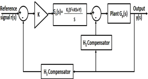
[image:2.595.308.549.48.177.2]For an nth-order LTI system such as (1), the deadbeat robust controller, as proposed in [12], is applied through the following two cell closed-loop control
Fig. 1. Basic structure of the robust deadbeat control loop
In this design, the system (1) is actuated by the following control law
5
where is the portion of the control signal generated by a cascade PID controller as follows
6
and is an output feedback control introduced by means of the following variable feedback gain
7
The error is defined as the difference between the reference input control and the output of an additional derivative controller
8
The structure of depends on the number of poles of the transfer function as follows
1 2
1 3 4
1 5
9
where equals the number of poles in transfer function. The cascade gain K is introduced in order to deal with higher-order plants, to compensate the nonlinearities, and to be able to independently specify the desired performances such as overshoot and settling time. The different parameters and gains in the control loop shown in Fig. 1. are determined by setting the characteristic equation of the equivalent closed-loop transfer function equal to the following deadbeat equation
⋯ 10
TABLE I
DEADBEAT COEFFICIENTS AND RESPONSE TIMES
Order np ′ ′
2nd 1.82 --- --- --- 3.47 4.82
3rd 1.90 2.20 --- --- 3.48 4.04
4th 2.20 3.50 2.80 --- 4.16 4.81
5th 2.70 4.90 5.40 3.40 4.84 5.43
′ and ′ are, respectively, the rise time and the settling time of the deadbeat step response. The normalized frequency is given as follows
11
where is the desired settling time, and is a positive constant generally selected to be 0.8 0.95.
B. Deadbeat Controller Implementation
First, the characteristic equation of the closed-loop transfer function is found from
1 12
which yields
13
Selecting the feedback as
1 ∑ 14
the development of (13) yields
∗ ∑
∗ ∑
∗ ∑
15
with
16
From (15), it is clear that to apply the deadbeat controller as proposed in [12], the orders higher than should be eliminated. This results in the following conditions
0 0 17
Hence, the relative degree of the system (4) should be . In other words, to apply the controller (5) to an arbitrary LTI system such as (1), an order-reduction or zero-cancellation phase is needed.
III. REALTIMECLOSED-LOOPCONTROLOFAN UAV
An UAV autopilot is designed to assure different levels of autonomy known as autopilot modes. These modes are classified into three categories [13]: 1-) standard modes such as manual, takeoff, land, and home modes, 2-) advanced modes such as targeting, deep stall, and PID modes, 3-) payload modes such as gimbal control and camera view modes.These autonomy capabilities allow the user to change autopilot behavior depending on the requested maneuvers.In addition, there is a pilot-in-the-loop mode which gives the user direct control of the aircraft using Radio Controlled (RC) mode for gain tuning, algorithm development, and cases where manual flight is required.
To be able to perform an autonomous flight, UAVs have to be tuned for different flight loops which are classified with respect to the relative degree as follows
Inner loops (=1): yaw rate, roll rate, and pitch rate. Outer loops (>1): roll, pitch, yaw, pitch-airspeed, throttle-airspeed, throttle-altitude, and pitch-altitude.
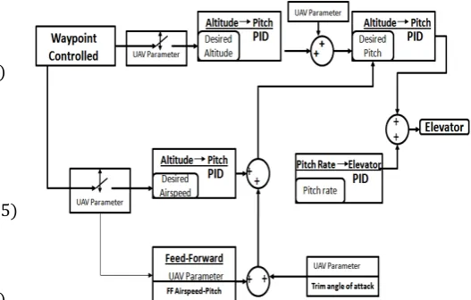
[image:3.595.287.551.433.601.2]Depending on the input-output relations, these loops are grouped into control blocks for which the control efforts are generated by cascading controllers using a combination of feedback and feedforward controls such as in Kestrel autopilot structure [13]. Assuming that all control blocks have access to the necessary sensor information, the following figure depicts the cascade structure of one of these blocks (Elevator-waypoints block control)
Fig. 2. Waypoint-elevator control block diagram of an UAV autopilot
IV. ROBUSTDEADBEATCONTROLLERDESIGN FORANUAVAUTOPILOT
In order to perform the control system design, it is necessary to start with an intended model of the system, and then proceed to the control design. Flight dynamics of fixed-wing aircrafts are well understood and reasonably extended to model the dynamics of UAVs which are characterized by a set of coupled and strongly nonlinear differential equations. However, under special circumstances and with specific assumptions such as straight steady flight and zero cross product, the use of small perturbation theory yields linear and decoupled into lateral and longitudinal equations of motion. In the present study, the longitudinal flight control of an UAV is considered for controller design and validation.
A. Longitudinal Flight Dynamics of an UAV
The longitudinal flight mode, is embodied by the X-force, Z-force, and pitch moment equations as follows
18
with
Θ 19
.2
.2 Θ
20
.2
. 2
21
22
and
̅
23
The variables and are the change of velocity components in x and z direction, respectively, is the steady state flight velocity, is the actual pitch angle, and
is the trim pitch angle. The matrix is the longitudinal flight matrix, and and are the aerodynamic and thrust control vector, respectively. The input and output variables are defined as follows
24
̅ 25
where and are elevator angle and thrust angle deflection, respectively.
B. Longitudinal Deadbeat Autopilot Design
In this section, the deadbeat controller derived above is analyzed in terms of agility and robustness against parameter uncertainties. The UAV model that we use here for control design and simulation is the model given in [10-11] for which the nominal pitch-axis transfer functions with respect to the elevator deflection are given as follows
̅
26
For a steady state flight velocity
12 / sec 472.44 / , the nominal system
transfer function ̅ ⁄ is given as follows
̅
1.423 0.134 1.839
0.02424 0.0683 0.1 0.0859 0.0836
27
The following figure depicts the open-loop time-domain response of (27) to a step unit elevator deflection
Fig. 3. Open-loop pitch angle response to a step unit elevator deflection.
In order to achieve the deadbeat system implementation requirements (17), the order reduction technique presented in [14] was used andseveral model reduction schemes were examined. The best results were obtained with the following reduced model
21.9976
The control objective is to assure a pitch angle path tracking with overshooting/undershooting less than 2%, maximum settling time of 2 second, and robustness against large parameter uncertainties. To successfully meet these performances, the proposed multistep design procedure is applied as follows.
First step: The cascade gain is set equal to 1 (the only tuning parameter) and the characteristic equation of the deadbeat transfer equation is constructed from table 1 with
4, 2 , 0.8 and 3.00625 / . Matching up this equation with (28) yields the following five nonlinear algebraic equations with six unknown design parameters
0.817 K ∗ 21.998 ∗ K 1 0.897 21.998K K 21.998K XK 6.614 1.028 21.998K 21.998K XK 21.998K YK 31.631
1 21.998ka 21.998K X 21.998K YK 76.074 21.998K Y 81.677
[image:5.595.314.528.61.419.2] [image:5.595.88.255.364.437.2]
Second step: The nonlinear algebraic equations above are solved for different values of . Test and selection process is conducted on the reduced system (28). The best results were obtained with the following design parameters
TABLE II
DEADBEAT DESIGN PARAMETERS FOR THE REDUCED SYSTEM Parameter Value
Kc 1.0000
X 1.4540 Y 3.7130
Ka 1.0390
K1 0.2478
K2 0.0083
Third step: The selected controller is now applied to the original system (26), and the cascade gain K is tuned until the desired performance requirements are achieved.
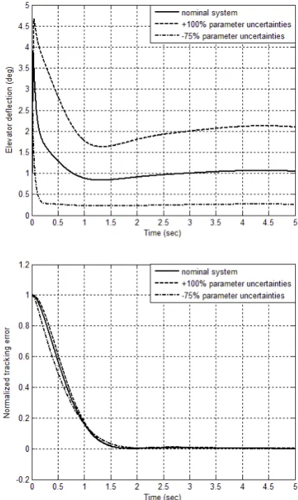
[image:5.595.302.549.536.598.2]To measure the efficiency and robustness of the controller, a desired pitch angle ̅ 22 is selected as illustration example. Computer simulations are conducted with nominal, +100% over-estimated, and 75% under-estimated system parameters. The following figures show the time-domain responses, control efforts, and tracking errors obtained
Fig. 4. Responses, control efforts, and tracking errors for an UAV pitch angle flight control system.
The following table summarizes the results of cascade gain tuning and time domain performances of the three systems above.
TABLE III
TIME-DOMAIN RESPONSES FOR DESIGN METHOD APPLIED TO NOMINAL AND UNCERTAIN SYSTEMS
Parameter uncertainties
K P.O [%]
P.U [%]
Tr90
[sec]
Ts [sec]
Nominal 0.77 0.00 0.55 1.134 1.472
100% increase 0.73 0.00 0.90 1.150 1.467
75% decrease 0.84 0.00 0.18 1.167 1.620
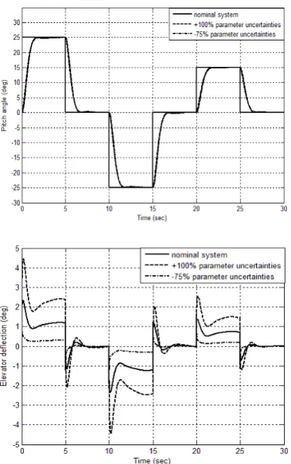
To check the ability of the designed controller to force an UAV to follow an arbitrary command, the same design parameter values shown in table 2 are used for an arbitrary pitch angle command pattern tracking. Again, the cascade gain K is tuned and the final values that correspond to the desired response are found to be as follows
TABLE IV
TIME-DOMAIN RESPONSES FOR DESIGN METHOD APPLIED TO PATH TRACKING WITH NOMINAL AND UNCERTAIN SYSTEMS
Parameter uncertainties
K P.O [%]
P.U [%]
Nominal 0.72 0.00 <1%
100% increase 0.70 0.00 <1%
[image:5.595.63.270.583.751.2] [image:5.595.340.516.728.788.2]The responses and needed control sequences for a pattern tracking mission are shown in the following figures
Fig. 5. Responses and control efforts for a pitch angle command sequence.
The results above show that a high closed-loop performance response with high robustness against large parameter uncertainties can be obtained with the proposed control framework. The designed deadbeat controller is also able to successfully perform tracking tasks under complex criteria within the limitations of system actuators.
V. CONCLUSION
A new strategy to design robust PID controller for uncertain higher-order systems is presented in this paper. The formal mathematical concepts of deadbeat control approach are developed and a new feature of robust deadbeat system is successfully implemented within an effective control framework. Computer simulations show that, for LTI systems, impressive time-domain performances and robustness to modeling uncertainties can be obtained with the proposed control strategy. Since the controller parameters are computed in advance and the tuning procedure is limited only to the cascade gain, the framework also provides an efficient and practical way for real-time PID parameter tuning.
REFERENCES
[1] O. A. A. Orqueda, X. T. Zhang, and R. Fierro, “An output feedback nonlinear decentralized controller for unmanned vehicle co-ordination,” International Journal Of Robust And Nonlinear Control. Int. J. Robust Nonlinear Control 2007; 17:1106–1128.
[2] M. Sadraey, R. Colgren, “Robust nonlinear controller design for a complete UAV mission,” AIAA Guidance, Navigation, and Control Conference and Exhibit 21 - 24 August 2006, Keystone, Colorado. [3] A. Benallegue1, A. Mokhtari, and L. Fridman, “High-order
sliding-mode observer for a quadrotor UAV,” International Journal Of Robust And Nonlinear Control Int. J. Robust Nonlinear Control. Copyright © 2007 John Wiley & Sons, Ltd.
[4] I. K. Nikolos, Kimon P. Valavanis, Nikos C. Tsourveloudis, and Anargyros N. Kostaras. “Evolutionary algorithm based offline/online path planner for UAV navigation,” IEEE Transactions On Systems, Man, And Cybernetics—Part B: Cybernetics, Vol. 33, No. 6, December 2003.
[5] I. K. Nikolos, N. Tsourveloudis, and K. P. Valavanis, “Evolutionary algorithm based 3-D path planner for UAV navigation,”in Proc. CD-ROM. 9th Mediterranean Conf. Control Automation, Dubrovnik, Croatia, 2001
[6] J. Z. Sasiadek and I. Duleba, “3-D local trajectory planner for UAV,” J. Intelligent Robotic Systems, vol. 29, pp. 191–210, 2000.
[7] A. C. Nearchou, “Adaptive navigation of autonomous vehicles using evolutionary algorithms,” Artif. Intell. in Eng., vol. 13, pp. 159–173, 1999.
[8] S. Kurnaz , O.Cetin , O.Kaynak, “Fuzzy logic based approach to design of flight control and navigation tasks for autonomous unmanned Aerial Vehicles,” J Intell Robot System, 54:229–244, 2009.
[9] Zelinski S, Koo T, Sastry S. “Optimization-based formation reconfiguration planning for autonomous vehicles,” Proceedings of the IEEE International Conference on Robotics and Automation, Taipei, Taiwan, September 2003; 3758–3763.
[10] K. Turkoglu, U. Ozdemir, M. Nikbay, E. Jafarov, “PID parameter optimization of a UAV longitudinal Flight control system,” World Academy of Science, Engineering and Technology 45, 2008. [11] K. Turkoglu, and E. M. Jafarov, “H inf. loop shaping robust control
vs. classical PI(D) control: A case study on the longitudinal dynamics of hezarfen UAV,” World Academy of Science, Engineering and Technology 45, 2008.
[12] J. Dawes, L. Ng, R. Dorf, and C. Tam, “Design of deadbeat robust systems,” Glasgow, UK, , pp1597-1598, 1994.
[13] Kestrel Autopilot System: User Guide, Copyright © 2004 – 2008. Procerus ® Technologies.