Initial Values in Estimation Procedures for State
Space Models (SSMs)
Raed Alzghool and Yan-Xia Lin
Abstract—In this paper, we will focus on State Space Models (SSMs), especially the stochastic volatility model, and look for a standard approach for assigning initial values in the Quasi-Likelihood (QL) and Asymptotic Quasi-Likelhood (AQL) estimation procedures.
Index Terms—State Space Models (SSMs), Quasi-Likelihood (QL), Asymptotic Quasi-Likelhood (AQL), Kalman filter, Non-linear and/or Non-Gaussian SSMs.
I. INTRODUCTION
T
HE class of state space models (SSM) provides a flexible framework for describing a wide range of time series in a variety of disciplines. For extensive discussion on SSM and their applications see Harvey [16] and Durbin and Koopman [13]. A state-space model can be written asyt=f1(αt, θ) +h1(yt−1, θ)ǫt, t= 1,2,· · ·, T (1)
where y1, . . . , yT represent the time series of observations;
θis an unknown parameter that needs to be estimated;f1(.)
is a known function of state variableαtandθ; and{ǫt} are
uncorrelated disturbances withEt−1(ǫt) = 0,V art−1(ǫt) =
σ2ǫ; in which Et−1, and V art−1 denote conditional mean
and conditional variance associated with past information updated to timet−1respectively. State variablesα1, . . . , αT
are unobserved and satisfy the following model
αt=f2(αt−1, θ) +h2(αt−1, θ)ηt, t= 1,2· · ·, T, (2)
where f2(.) is a function of past state variables and θ;
{ηt} are uncorrelated disturbances with Et−1(ηt) = 0,
V art−1(ηt) =ση2.h1(.)andh2(.)are unknown functions.
One special application that we will consider in detail is the Stochastic Volatility Model (SVM), a frequently used model for returns of financial assets. Applications, together with estimation for SVM, can be found in Jacquier, et al [22]; Briedt and Carriquiry [8]; Harvey and Streible [19]; Sandmann and Koopman [27]; Pitt and Shepard [25].
There are several approaches in the literature for esti-mating the parameters in SSMs by using the maximum likelihood method when the probability structure of under-lying model is normal or conditional normal. Durbin and Koopman ([14], [13]) obtained accurate approximation of the log-likelihood for Non-Gaussian state space models by using Monte Carlo simulation. The log-likelihood function is maximised numerically to obtain estimates of unknown parameters. Kuk [23] suggested an alternative class of esti-mate models based on conjugate latent process and applied
Manuscript received March 04, 2011; revised XXXX XX, 2011. R. Alzghool is with the Department of Applied Science, Faculty of Prince Abdullah Ben Ghazi for Science and Information Technology, Al-Balqa’ Applied University, Al-Salt, Jordan e-mail: [email protected] .
Y. Lin is with School of Mathematics and Applied Statistics, Uni-versity of Wollongong, Wollongong, NSW 2500, Australia e-mail: [email protected] .
it to approximate the likelihood of a time series model for count data. To overcome the complex likelihoods of a time series model with count data, Chan and Ledolter [10] proposed the Monte Carlo EM algorithm that uses a Markov chain sampling technique in the calculation of the expectation in the the E-step of the EM algorithm. Davis and Rodriguez-Yam [12] proposed an alternative es-timation procedure which is based on an approximation to the likelihood function. Alzghool and Lin [2] proposed quasi-likelihood (QL) approach for estimation of state space models without full knowledge on the probability structure of relevant state-space system. The QL method relaxes the distributional assumptions and only assumes the knowledge on the first two conditional moments ofytandαtassociated
past information. This weaker assumption makes the QL method widely applicable and become a popular method of estimation. A comprehensive review on the QL method is available in Heyde [21]. A limitation of the QL is that in practice, the conditional second moments of of yt and
αt might not available. The AQL approach provides an
alternative method of parameter estimation when unknown form of heteroscedasticity is presented.
The estimation procedure for SSMs consists of two parts. The first part is, given observations{y1, . . . , yT}, to estimate
state variables αt. The second part is to combine the
infor-mation of{yt} and{αˆt} to estimate unknown parameter θ
in the model. The Kalman filter and the smoother methods are widely used to estimate an unobservable series, state variables, in SSMs (Anderson and Moore [7], Harvey [17]). In summary, the QL and AQL estimating procedures discussed in Alzghool and Lin ([2],[3], [5]), Alzghool [4], and Alzghool, et al [6]. consist of the following steps:
(i) Assign initial values toα0,θ0 andΣ0=I.
(ii) Obtain the QL/AQL estimates αˆt of αt for t =
1,2, . . . , T.
(iii) For the AQL estimating procedure, obtain Σˆt,n by
using the kernel method.
(iv) Obtain the QL/AQL estimateθˆof θ.
(v) Steps (ii), (iii) and (iv) will be alternatively repeated until estimates converge.
The final estimation results for SSMs might be jointly af-fected by the initial valuesα0andθ0which initially assigned
to the underlying model during the inference procedure. In this paper, following two issues are investigated. (1) How sensitive are the final estimates to the initial values assigned to the state variableα0 andθ0?
(2) If the estimation results are sensitive to the choice of the initial values, what should initial value of the state variableα0be and how is the final estimate ofθdetermined?
via simulation studies. In Section III, a new suggestion for choosing the initialisation of the state variable α0 is given.
In Section IV, the impact of the starting values of system parameters θ0 in the estimation results is investigated via
simulation studies. In Section V, a standard procedure to improve the grid search procedure for obtaining a better estimation of θis established. In Section VI applications of the QL and AQL methods to real data modelled by SSMs are given. In Section VII, a conclusion is provided.
II. EFFECT OFINITIALISATION OFα0
The impact of the initial value of the state variableα0 on
the final inference result is illustrated via simulation studies in this section. Simulation study based on stochastic volatility model (SVM) is presented below.
A. Stochastic Volatility Models (SVM)
Consider the stochastic volatility model,
ln(yt2) =αt+ lnξt2, t= 1,2,· · ·, T, (3)
αt=γ+φαt−1+ηt, t= 1,2,· · ·, T, (4)
where both ξt and ηt are i.i.d. r.v.’s; ηt has mean 0 and
variance ση2.
In order to show how the initial valueα0 effects the final
estimation in the SVM when the QL and AQL approaches are applied, we carried out a simulation study on SVM Model defined by (3) and (4). The simulation was conducted as follows. First, 1,000 independent samples of size 500 are generated from (3) and (4) based on a true parameter θ = (γ, φ), where ηt ∼N(0, ση2), ξt ∼N(0,1), and the initial
value for α0 in the true model is α0 = 0. Once{yt} and
{αt} are generated, pretend that {αt} is unobserved and γ,
andφare unknown. Then apply the QL and AQL estimation procedures to{yt} only to obtain the estimate ofαt,γ, and
φ. Different parameter settings for(γ, φ, σ2
η)are considered
in the simulation. The mean and root mean squared errors for ˆ
γandφˆbased on 1,000 independent samples are calculated. Letαˆ0be the initial state used in the inference procedure.
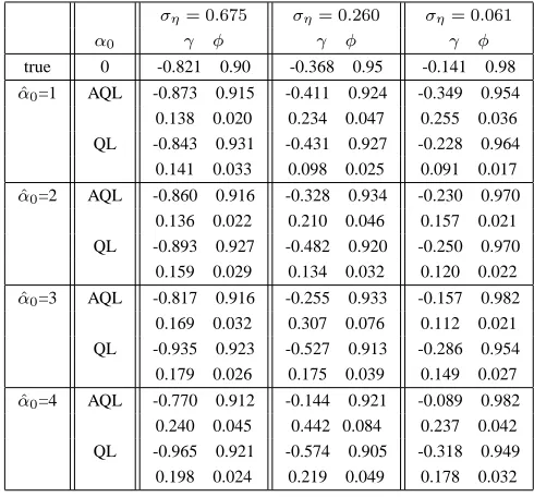
In Table I, different values of αˆ0, mean and root mean
squared errors for γˆ, and φˆ given by the QL and AQL methods are reported.
We can see from Table I that the RMSE of QL and AQL estimates are increased when αˆ0 is chosen farther from the
true value α0. Since the increase in the RMSE for QL is
less than for AQL, this indicates that the QL approach is less sensitive to the initial value of state variable than the AQL approach.
III. DETERMINATION OFαˆ0
Consider the univariate time seriesyt satisfying
yt=αt+ǫt, t= 1,2,· · ·, T (5)
αt=αt−1+ηt, t= 1,2,· · ·, T (6)
whereǫt∼N(0, σ2ǫ),ηt∼N(0, σ2η), andα0∼N(a0, P0).
{ǫt} and {ηt} are two independent Gaussian white noise
series. The initial valueα0 is independent of{ǫt}and{ηt}
[image:2.595.303.548.98.326.2]for t >0. In literature,αt is referred to as the trend of the
TABLE I
QLANDAQLESTIMATES,BASED ON1,000REPLICATIONS. THE ROOT MEAN SQUARE ERROR OF EACH ESTIMATE IS REPORTED BELOW THAT ESTIMATE,BASED ON DIFFERENT INITIAL VALUES FORα0(T = 500).
ση= 0.675 ση= 0.260 ση= 0.061
α0 γ φ γ φ γ φ
true 0 -0.821 0.90 -0.368 0.95 -0.141 0.98
ˆ
α0=1 AQL -0.873 0.915 -0.411 0.924 -0.349 0.954 0.138 0.020 0.234 0.047 0.255 0.036 QL -0.843 0.931 -0.431 0.927 -0.228 0.964 0.141 0.033 0.098 0.025 0.091 0.017
ˆ
α0=2 AQL -0.860 0.916 -0.328 0.934 -0.230 0.970 0.136 0.022 0.210 0.046 0.157 0.021 QL -0.893 0.927 -0.482 0.920 -0.250 0.970 0.159 0.029 0.134 0.032 0.120 0.022
ˆ
α0=3 AQL -0.817 0.916 -0.255 0.933 -0.157 0.982 0.169 0.032 0.307 0.076 0.112 0.021 QL -0.935 0.923 -0.527 0.913 -0.286 0.954 0.179 0.026 0.175 0.039 0.149 0.027
ˆ
α0=4 AQL -0.770 0.912 -0.144 0.921 -0.089 0.982 0.240 0.045 0.442 0.084 0.237 0.042 QL -0.965 0.921 -0.574 0.905 -0.318 0.949 0.198 0.024 0.219 0.049 0.178 0.032
series, which is not directly observable, andytis observable.
The model is called a local level model in Durbin and Koopman ([13], Chapter 2), which is a simple case of the
structural time series model of Harvey [17].
When nothing is known about the initial valueα0, the
ini-tialisation ofα0 is usually given by a diffuse prior approach
that fixesa0 at an arbitrary value and letP0→ ∞(Zivot et
al. [30], Durbin and Koopman [13], Harvey [16]). However,
some researchers consider that the diffuse approach is not realistic because they regard that the assumption of infinite variance is unnatural, given that all observed time series have finite values. From this point of view an alternative approach is suggested, which assumes thatα0 is an unknown constant
and needs to be estimated from the data. In Harvey [18], it is suggested that the initial value of α0 can be taken as
y1. This is the same value as that obtained by assuming
that α0 is diffuse. More details about the intitialisation of
the Kalman filter under the normality assumption for SSM are provided in Durbin and Koopman ([13], Chapter 5 and references therein). Several other suggestions on initialisation for the state variable in SSM under normality assumption are given in a recent survey by Casals and Sotoca [9]. They derived an exact expression for the conditional mean and variance of the initial state of SSM.
In this paper, we follow the QL method to derive a simple method for determiningαˆ0without assigning any probability
distribution toα0.
Consider the following state-space model:
yt=f(αt, θ) +ǫt, t= 1,2,· · ·, T, (7)
αt=g(αt−1, θ) +ηt, t= 1,2· · ·, T. (8)
Fort= 1, we have
y1=f(α1, θ) +ǫ1, (9)
In models (9), and (10),α1,α0,ǫ1, andη1 are unobserved.
Assume θis known or determined by empirical knowledge. The rule used to determine αˆ0 should meet the condition
that given observation y1,αˆ0 is able to ensure thatf(ˆα1, θ)
is an optimal estimation of E(y1).
From (9), consider
ǫ1=y1−f1(α1, θ)
Let α1 be an unknown parameter and consider estimating
function space
G(1)T ={a1(y1−f1(α1, θ)) | a1∈R}.
A standardised optimal estimating function inGT(1) is
G∗
(1)(α1) =−E(
∂f ∂α1
)[V ar(ǫ1)]−1(y1−f(α1, θ)).
If E(∂α∂f1)6= 0, and f
−1 exists, the optimal estimator of
α1 will be given byG∗(1)(α1) = 0, that is,
ˆ
α1=f−1(y1, θ). (11)
Using (10), consider
η1=α1−g(α0, θ).
Let α0 be an unknown parameter and consider estimating
function space
GT(0)={a0(α1−g(α0, θ)) | a0∈R}.
A standardised optimal estimating function inGT(0) is
G∗
(0)(α0) =−E(
∂g
∂α0)[V ar(η1)]
−1(α
1−f(α0, θ)).
IfE(∂α∂g0)6= 0, andg−1 exists, the optimal estimator ofα 0
will given by G∗
(0)(α0) = 0, that is,
ˆ
α0=g−1(α1, θ). (12)
Therefore, we make the following suggestion for determining the initial stateαˆ0 in inference process.
Suggestion: For a SSM
yt=f(αt, θ) +ǫt, t= 1,2,· · ·, T
αt=g(αt−1, θ) +ηt, t= 1,2· · ·, T.
IfE(∂α∂f1)6= 0,E(∂α∂g0)6= 0,f−1andg−1exist, the optimal
decision onαˆ0 is
ˆ
α0=g−1(f−1(y1)). (13)
For convenience, denote this αˆ0 as αˆ∗0.
As an example for (5) and (6), the optimal value for αˆ0
is y1, which is the same as the one given under diffuse
conditions.
In the following, we apply the Suggestion to stochastic volatility model, and use simulation to investigate whether the Suggestion is practicable or not.
TABLE II
QLANDAQLESTIMATES BASED ON1,000REPLICATION. THE ROOT MEAN SQUARE ERROR OF EACH ESTIMATE IS REPORTED BELOW THAT
ESTIMATE.αˆ∗
0IS DIFFERENT FROM SAMPLE TO SAMPLE. (T = 500).
ση= 0.675 ση= 0.260 ση= 0.061
α0 γ φ γ φ γ φ
true 0 -0.821 0.90 -0.368 0.95 -0.141 0.98 α0=0 AQL -0.878 0.92 -0.499 0.91 -0.437 0.94 0.136 0.019 0.229 0.049 0.354 0.052 QL -0.788 0.94 -0.391 0.94 -0.198 0.97 0.140 0.037 0.071 0.019 0.063 0.013 α0=αˆ∗
0 AQL -0.857 0.92 -0.499 0.91 -0.440 0.94 0.163 0.024 0.243 0.051 0.402 0.060 QL -0.830 0.93 -0.378 0.94 -0.194 0.97 0.142 0.034 0.082 .019 0.071 .014
A. Stochastic Volatility Model
Consider stochastic volatility process defined by (3) and (4), i.e.
ln(y2
t) =αt+ lnξt2, t= 1,2,· · ·, T.
αt=γ+φαt−1+ηt, t= 1,2,· · ·, T,
where both ξt and ηt are i.i.d. r.v.’s; ηt has mean 0 and
varianceσ2 η,φ6= 0.
Let
ǫ1= lnξ12−E(lnξ12).
Using (3) and (4), it follows that
ǫ1 = ln(y12)−α1−E(lnξ12)
= ln(y12)−f(α1, θ),
and
η1 = α1−(γ+φα0)
= α1−g(α0, θ),
where θ = (γ, φ)′, f(α
1, θ) = α1 + E(lnξ12), and
g(α0, θ) =γ+φα0.
SinceE(∂α∂f1) = 16= 0,E(∂α∂g0) =φ6= 0, andf−1, g−1
exist, therefore,
ˆ α∗
0=g−1(f−1(y1)) =
ln(y2
1)−E(lnξ12)−γ
φ . (14)
If ξt has standard normal distribution, then E(lnξt2) =
−1.2704 and V ar(lnξ2
t) = π2/2 (see Abramowitz and
Stegun [1], p. 943). Then, substituting in (14)
ˆ α∗
0=g−1(f−1(y1)) =
ln(y2
1) + 1.2704−γ
φ . (15)
To show how the optimal initial valueαˆ∗
0 effects the final
estimation when the QL and AQL approaches are applied, we carried out a simulation study on SVM model defined by (3) and (4). We camper the estimation of (,φ) given by the trueα0 andαˆ∗0. Results are presented by Table II.
Table II shows that, compared to results in Table I, the estimation given by αˆ∗
0 are close related to those given by
Fig. 1. Histogram of QL estimation ofγin SVM, based on 2,000 different starting values.
IV. THESTARTINGVALUES FORSYSTEMPARAMETERθ0
In this section, we consider the starting value for system parametersθ0. As described in literature, the outputs of
non-linear inference procedures rely strongly on the appropriate value of the initial parameter θ0. It is usually suggested
that θ0 should be chosen from a close neighbourhood of
its true value (Zivot et al. [30]). Since the true value of θ0 is unknown, it is an issue how to identify the close
neighbourhood of θ0.
The impact of the starting values of system parametersθ0
is illustrated via simulation studies below.
A. Stochastic Volatility Models
Consider SVM as given in (3) and (4) where ηt ∼
N(0,0.6752), ξ
t ∼N(0,1), and the initial value for α0 in
the true model is given byα0= 0. In this example, the state
space model is involved with the parameter θ= (γ, φ). Let θ= (−0.368,0.95), a sequence of observationsy1,· · ·, y1000
from the state space model were generated. Then we pre-tend θ is unknown. Consider a two-dimensional range (-0.868,0.132; 0.80,0.99) forθ= (γ, φ), which covers the true parameter (-0.368,0.95). Then we apply a two-dimensional grid search to (-0.868,0.132; 0.80,0.99) with increasment of 0.01. For each starting value ofθfrom the grid area, we apply the QL and AQL estimating procedures to the realisation y1,· · ·, y1000 and obtain the QL and AQL estimation of θ
where αˆ0 = α0 are used. In Figure 1 - 4, we show the
histograms of QL and AQL estimation of γandφbased on 2000 different starting values.
Like others estimation procedures described in literature, the QL and AQL estimations ofθrely strongly on the value of the initial parameterθ0.
We note an interesting phenomenon in the histograms illustrated in Figures 1 - 4. The true value of a parameter is not always allocated in the low frequency area. Obviously, the size of the low frequency area relies on the nature of the true model. This suggests that, although it is not appropriate to quantitatively identify an optimal estimation on system parameters utilising the information provided by a histogram diagram indirectly through the grid search approach, it is possible to narrow down and obtain a potential
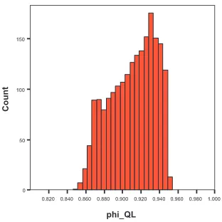
[image:4.595.88.240.70.227.2]Fig. 2. Histogram of QL estimation ofφin SVM, based on 2,000 different starting values.
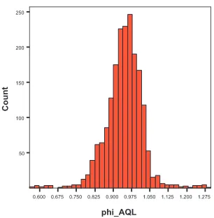
Fig. 3. Histogram of AQL estimation ofγin SVM, based on 2,000 different starting values.
Fig. 4. Histogram of AQL estimations of φin SVM, based on 2,000 different starting values.
[image:4.595.344.498.71.225.2] [image:4.595.344.497.296.455.2] [image:4.595.342.497.524.684.2]V. DETERMINATION OF THEESTIMATION OF THE
SYSTEMPARAMETERθ
In their survey article, Zivot et al. [30] suggested choosing a starting valueθ0close to the true value ofθ. The estimation
of θ using a Monte Carlo approximation for count data given by Kuk [23] is only good when the initial value of θ is assigned around the true value of θ. Other approaches to decide θ0 are also suggested in literatuer. For example,
Durbin and Koopman [14] numerically maximised the ap-proximate likelihood for non-Gaussian SSMs to obtain the starting value for θ0; Sandmann and Koopman [27] used a
two-dimensional grid search procedure which searches for an appropriate starting value for θ0 across the surface of a
Gaussian log-likelihood function; Geweke and Tanizaki [15] and Tanizaki and Mariano ([28], [29]) used a simple grid search for θ0 where the expected log-likelihood function is
maximised.
The ML method is a popular method for estimating the parameters of SSMs. The ML method works if the probabil-ity structure of the underlying state space system is known. In practice, it is not realistic to assume that the system’s probability structure is known. Then, the maximum likeli-hood method becomes impracticable. Therefore, searchingθ0
based on maximising the log-likelihood function cannot be applied. Without knowledge of the log-likelihood, a distribu-tion free procedure can be considered. It is implemented by a grid search over a feasible region of the parameter space, and the parameter estimation will be the one giving the minimum residual sum of squares (RSS)( see Coakley et al. [11] and Naik-nimbalkar and Rajarshi [24]).
In this paper, we adapt grid search procedure but with some improvements. It is sensible to obtain the estimate of θ by utilising a the grid search, and the residual sum of squares. However, if the grid search area is relatively large, the smallest sum of residuals might not lead to the best estimation of θ. One example can be fond from the simulation study discussed below. To improve the outcomes of the grid search procedure and sum of residuals, we need to reduce the area of the grid search into a reasonable size. We suggest the following steps in determining the esti-mation of θ for SSMs: (in the following, we used a two-dimensional parameter as an example.)
Step 1. First determine a reasonable range. Based on experience, this range should cover the true parameterθ. For example, for PM and SVM, decide a two-dimensional area [a,b; c,d], covering the true parameterθ.
Step 2. Following the two-dimensional grid search proce-dure, we assignθ0with a different starting value, and obtain
the QL or AQL estimation of the parameter.
Step 3. Draw the histogram of the QL or AQL estimates obtained from step 2.
Step 4. Consider the region with the highest frequency estimation values in the histogram as a potential region to cover the true value of the parameter. Obviously this potential region tends to be smaller than the range in Step 1.
Step 5. Letyˆt(ˆθ)be the predicted value ofytbased on the
observation equation. Find θˆ, which minimises RSSy(θ) =
PT
t=1(yt−yt(ˆθ))2 in the potential region.
The above steps used to determine the estimate of θ for SSMs are illustrated by the following example.
TABLE III
QL, AQL,QL∗,ANDAQL∗ESTIMATES,ANDRSS
yARE REPORTED
BELOW EACH ESTIMATE.
SVM ση= 0.675
γ φ
true 0 -0.363 0.95
AQL -0.30 0.95
RSSy 323.53
QL -0.45 0.93
RSSy 660.62
AQL∗ -0.31 0.94
RSSy 457.65
QL∗ -0.32 0.95
RSSy 725.03
Example : Consider SVM as given in (??) and (??),
where ηt ∼ N(0,0.6752), ξt ∼ N(0,1), and the initial
value for α0 in the true model is given by α0 = 0. In
this example, the state space model is involved with the parameterθ= (γ, φ). Letθ= (−0.368,0.95), a sequence of observationsy1,· · ·, y1000 andα1,· · ·, α1000from the SVM
were generated. Then we pretend{αt} andθare unknown.
Step 1. Consider a two-dimensional range (-0.868,0.122; 0.80,0.99) forθ = (γ, φ), which covers the true parameter (-0.368,0.95).
Step 2. Apply a two-dimensional grid search to (-0.868,0.122; 0.80,0.99) with increases of 0.01. For each starting value ofθfrom the grid area, we apply the QL/AQL estimating procedures and obtain the QL/AQL estimate ofθ. Step 3. In Figures 1-4, we show the histograms of the QL and AQL estimates ofγandφ, based on 2,000 different starting values.
Step 4. From the histograms of the QL estimates of γ and φ given in Figures 1 and 2, the potential region for parameter (γ, φ) is chosen as [-0.36,-0.12; 0.91,0.95]. By using the histogram of the AQL estimates of and φ given in Figures 3 and 4, the potential region for parameter(γ, φ) is chosen as [-1.0,-0.30; 0.80,0.95].
Step 5. Find the estimate of γ and φ by minimising the residual sum of squares (RSSy(θ)) in the potential region
and give the QL estimate of θ (-0.32,0.95), and the AQL estimate ofθ (-0.31,0.94).
In Table III, the QL and AQL denote the estimation ofθ, which gives the smallest RSSy based on the region given
in Step1, and the QL∗ andAQL∗ denote the estimates of θ, which gives the smallest RSSy based on the potential
region determined in Step 4. We can see from Table III, that the estimate ofθ has improved in all cases after using the potential region determined by the information provided by histogram diagram. The above examples indicate that using the potential region is able to significantly improve the performance ofRSSy.
VI. REAL DATA APPLICATION
In this section, we consider log returns of Pound/Dollar exchange rates. The data are the daily observation of weekdays’ closing pound to dollar exchange rates xt
been studied and analysed by Harvey et al. [20], Davis and Rodriguez-Yam [12]; Rodriguez-Yam [26]; Durbin and Koopman [13] and Alzghool and Lin [2].
Let yt = log(xt/xt−1), t = 1,2,· · ·,945. To model yt,
we adopt the same SVM used by Davis and Rodriguez-Yam [12].
yt=σtξt=eαt/2ξt, t= 1,2,· · ·,945, (16)
αt=γ+φαt−1+ηt, t= 1,2,· · ·, T, (17)
where both ξt and ηt are i.i.d. r.v.’s; ηt has mean 0 and
variance σ2
η. Therefore,
ln(yt2) =αt+ lnξt2, t= 1,2,· · ·, T. (18)
If ξt were standard normal, then E(lnξt2) = −1.2704 and
V ar(lnξ2
t) =π2/2(see Abramowitz and Stegun [1], p. 943).
Letǫt= lnξt2+ 1.2704, andδt= (ǫt, ηt)′.
We apply the QL method to the data model under the assumption that the conditional covariance matrix is known as follows:
V art−1(δt) =Σt=
π2
2 0
0 σ2 η
.
The AQL method is applied to the data by assuming no knowledge of the conditional covariance matrix. In the QL approach, ση will estimate from the residuals, but in AQL
approach it is estimated by the Kernel estimator.
Following steps are for obtaining the estimate of θ = (φ, γ)for the Pound/ Dollar exchange rate data:
Step 1. Decide a grid search area, based on previous studies: (-0.813,0.177; 0.80,0.99).
Step 2. Apply a two-dimensional grid search to (-0.813,0.177; 0.80,0.99) with increases of 0.01. For each starting value ofθfrom the grid area, we apply the QL/AQL estimating procedures and obtain the QL/AQL estimate ofθ. Step 3. In Figures 5-8, we show the histograms of the QL and AQL estimates ofγandφ, based on 2,000 different starting values.
Step 4. From the histograms of the QL estimates of γ and φ given in Figures 5 and 6, the potential region for parameter (γ, φ) is chosen as (-0.17,-0.04; 0.86,0.95). By using the histogram of the AQL estimates of γandφgiven in Figures 7 and 8, the potential region for parameter(γ, φ) is chosen as (-0.45,0.1; 0.825,0.99).
Step 5. Find the estimate of γ andφ by minimising the residual sum of squares (RSSy(θ)) in the potential region
[image:6.595.341.497.69.225.2]and the QL estimate of θ is (-0.048,0.949), and the AQL estimate of θ is (-0.082,0.971).
Table IV shows estimations ofθ= (φ, γ)obtained by dif-ferent methods. AQL denotes the asymptotic quasi-likelihood estimate, QL the estimate obtained by quasi-likelihood ap-proach, AL the estimate obtained by maximising the approx-imate likelihood proposed by Davis and Rodriguez-Yam [12] and MCL the estimate obtained by maximising the estimate of the likelihood proposed by Durbin and Koopman [14]. AL and MCL outputs are taken from Rodriguez-Yam [26].
In Table IV, the estimate of γ and φ by QL, AL and MCL are close to each other. These three methods are carried out under the same assumption where ξt and ηt
[image:6.595.344.500.291.447.2]are independent. This might indicate that the performance of QL, AL and MCL will be similar. However, the AQL
[image:6.595.342.497.510.667.2]Fig. 5. Histogram of QL estimates ofγin SVM, based on 2,000 different starting values.
Fig. 6. Histogram of QL estimates ofφin SVM, based on 2,000 different starting values.
Fig. 7. Histogram of AQL estimates ofγin SVM, based on 2,000 different starting values.
estimates are slightly different from those of QL, as well as the estimates of AL and MCL.
Fig. 8. Histogram of AQL estimates ofφin SVM, based on 2,000 different starting values.
TABLE IV ESTIMATES OFγ,φANDσ2
ηFORPOUND/DOLLAR EXCHANGE RATE
DATA.
ˆ
γ φˆ σˆ2
η
AQL -0.082 0.971 0.239 QL -0.048 0.949 0.025 AL -0.023 0.957 0.026 MCL -0.023 0.975 0.027
does not. To understand which model setting is appropriate, it requires checking whether we can acceptcov(ηt, ξt) = 0.
We considerˆǫtandηˆtgiven by QL and find thatˆǫtandηˆtare
highly correlated withr= 0.91and significant at level 0.01. So, the assumption of ǫt and ηt uncorrelated is not valid.
Therefore, it is not appropriate to apply the QL method to the data. Thus, we rather accept the estimations given by the AQL method than those given by the QL method.
VII. CONCLUSION
In this paper, we investigated the sensitivity of the QL and AQL estimation procedures to initial values assigned to state variableα0andθ0via simulation studies. A suggestion
on choosing the initial value of state variable α0, without
knowing the system’s probability structure has been given. Simulation studies indicate that it is relatively reliable to follow the suggestion in determining the initialisation of the state variableα0during inference procedure. Apart from the
impact ofα0, the QL and AQL estimates ofθalso sensitive to
the value of the starting parameterθ0. In literature, it always
suggestes that θ0 has to be chosen from a neighbourhood
close to the true value ofθ. But, it dose not mention how to determine the close neighbourhood given the location of the true θ is unknown. In this paper, we established a standard procedure for determing the ”close neighbourhood” and the estimation ofθ in terms of minimizingRSSy.
REFERENCES
[1] M. Abramovitz, and N. Stegun, Handbook of Mathematical Functions, Dover Publication, New York, 1970.
[2] R. Alzghool and Y.-X. Lin, Asymptotic Quasilikelihood Based on Ker-nel Smoothing for Nonlinear and Non-Gaussian State-Space Models, ICCSDE, London, UK, pp. 926-932, WCE 2007.
[3] R. Alzghool and Y.-X. Lin, Parameters Estimation for SSMs: QL and AQL Approaches, IAENG International Journal of Applied
Mathemat-ics, 38, pp. 34-43, 2008.
[4] R. Alzghool, Estimation for state space models: quasi-likelihood and asymptotic quasi-likelihood approaches, PhD thesis, School of Math-ematics and Applied Statistics, University of Wollongong, Australia, 2008.
[5] R. Alzghool and Y.-X. Lin, Estimation for State-Space Models: Quasi-likelihood, Proceedings of the Tenth Islamic Countries Conference on
Statistical Sciences (ICCS-X), Volume I, The Islamic Countries Society
of Statistical Sciences, Lahore: Pakistan, pp. 409-423, 2010.
[6] R. Alzghool and Y.-X. Lin, and S. X., Chen, Asymptotic Quasi-likelihood Based on Kernel Smoothing for Multivariate Heteroskedas-tic Models with Correlation, American Journal of MathemaHeteroskedas-tical and
Management Sciences,(accepted), 2010.
[7] B. D. O. Anderson and J. B. Moore. Optimal Filtering, Prentice-Hall, New York, 1979.
[8] F.J. Breidt, and A.L. Carriquiry, Improved quasi-maximum likelihood estimation for stochastic volatility models. In: Zellner, A. and Lee, J.S. (Eds.), Modelling and Prediction: Honouring Seymour Geisser, Springer, New York, 228-247, 1996.
[9] J. Casals and S. Sotoca, Exact initial condition for maximum likelihood estimation of state space models with stochastic inputs, Economics
Letters, 57, 261-267, 1997.
[10] K. S. Chan and J. Ledolter, Monte Carlo EM estimation for time series models involving counts, J. Amer. Statist. Assoc., 90, 242-252, 1995.
[11] J. Coakley, A. Fuertes, and Perez, Numerical issues in threshold autoregressive modeling of time series, Journal of Economic Dynamics
Control, 27, 2219-2242, 2003.
[12] R. A. Davis, and G. Rodriguez-Yam, Estimation for State-Space Models: an approximate likelihood approach, Statistica Sinica, 15, 381-406, 2005.
[13] J. Durbin, and S. J. Koopman, Time Series Analysis by State Space
Methods, Oxford, New York, 2001.
[14] J. Durbin, and S. J. Koopman, Monte Carlo maximum likelihood estimation for non-gaussian state space models, Biometrika, 84, 669-684, 1997.
[15] J. Geweke and H. Tanizaki, On Markov Chain Monte Carlo methods for nonlinear and non-Gassian state-space models, Comm. Statist.
Simulation Comput., 28, 867-894, 1999.
[16] A. C. Harvey, Forecasting, Structural Time Series Moodels and the
Kalman Filter, Cambridge University Press, 1989.
[17] A. C. Harvey, Forecasting, Structural Time Series Moodels and the
Kalman Filter, Cambridge University Press, 1994.
[18] A. C. Harvey, Forecasting with unobserved components time series models, volume 1 of Handbook of Economic Forecasting, chapter 7, pages 328-408. ELSEVIER B. V., 2006.
[19] A. C. Harvey, and M. Streible, Testing for a slowly changing level with special reference to stochastic volatility, J. Econometrics, 87, 167-189, 1998.
[20] A. Harvey, E. Ruiz, and N. Shephard, Multivariate stochastic variance models, Review of Economic Studies, 61, 247-264, 1994.
[21] C. Heyde, Quasi-likelihood and its Application: a general Approach
to Optimal Parameter Estimation, Springer, New York, 1997.
[22] E. Jacquire, and N. G. Polson, and P. E. Rossi, Bayesian analysis of stochastic volatility models ( with discussion), J. Bus. Econom. Statist,
12, 371-417, 1994.
[23] A. Y. Kuk, The use of approximating models in Monte Carlo maximum likelihood estimation, Statist. Probab. Letter, 45, 325-333, 1999. [24] U. V. Naik-nimbalkar and M. B. Rajarshi, Filtering and smoothing
via estimating functions, Journal of American statistical Association,
90,(429),301-306, 1995.
[25] M. K. Pitt, and N. Shepard, Filtering via simulation: auxiliary particle filters, J.Amer. Statist. Assoc., 94, 590-599, 1999.
[26] G. Rodriguez-Yam, Estimation for State-Space Models and Baysian
regression analysis with parameter constraints, Ph.D. Thesis, Colorado
State University, 2003.
[27] G. Sandmann, and S. J. Koopman, Estimation of stochastic volatility models via Monte Carlo maximum likelihood, J. Econometrics, 87, 271-301. 1998.
[28] H. Tanizaki and R. S. Mariano, Prediction, fltering and smoothing in nonlinear and nonnormal cases using Monte-Carlo integration, J. of
App. Econo- metrics, 9(2), 163-179, 1994.
[29] H. Tanizaki and R. S. Mariano, Nonlinear and non-Gaussian state-space modeling with Monte-Carlo simulation, J. of Econometrics, 83, 263-290, 1998.
[30] E. Zivot, J. Wang, and S. J. Koopman, State Space and Unobserved Com- ponent Models: Theory and Application, chapter State space
modelling in macroeconomics and finance using SsfPack, 284-335,
[image:7.595.87.240.69.225.2]