Abstract—Efficient and effective supplier selection and order allocation are important issues to be considered for designing flexible and highly competitive supply chains which maximize the manufacturer’s total profit and ensure stable material flows. This paper proposes a novel methodology for solving an integrated supplier selection and order allocation problem that arises in the design of a multi-product supply chain, with particular reference to the influence of customer flexibility. A new mixed integer programming model incorporating the characteristics of the problem is developed to assist the manufacturer in the decision making processes. Due to the complexity and the NP-Hard nature of the proposed model, a novel hybrid algorithm based on the strengths of constraint programming (CP) and simulated annealing (SA) is developed to solve this challenging problem. The performance of the proposed algorithm is tested with a set of randomly generated test problems. Comparison with the computational results obtained by ILOG OPL clearly shows that the hybrid algorithm can locate profit-effective solutions with less computational efforts.
Index Terms—Constraint programming, customer flexibility, simulated annealing, supplier selection, order allocation
I. INTRODUCTION
ITH increasing product variety and escalating demand volatility, maintaining an efficient and flexible supply chain has become more critical for most enterprises. In addition, it has been observed that customers are often indifferent to certain product specifications and are often willing to accept less desirable products given certain price discounts [7]. This flexible customer behavior brings additional degree of freedom in promising customer orders and arranging available production resources. Indeed, the purpose of achieving high service level and low manufacturing cost in such dynamic supply chain environment imposes a major challenge in the order commitment process, which mainly consists of supplier selection and order allocation problems.
In this connection, this paper takes a new perspective to tackle the challenge of matching various customer
Manuscript received March 6, 2011.
K.L.Mak is Professor at the Department of Industrial and Manufacturing Systems Engineering, The University of Hong Kong.(phone:(852) 28592582; e-mail: [email protected]).
L.X.Cui is currently a PhD student at the Department of Industrial and Manufacturing Systems Engineering, The University of Hong Kong. (e-mail: [email protected]).
requirements and available production resources in a multi-product supply chain by integrating customer flexibility into the order commitment process. The objective is to propose a novel methodology to assist the manufacturer in deciding the production quantities of all the product variants and the corresponding order allocations among selected suppliers. A new mathematic model in the form of a mixed integer programming (MIP) model is firstly developed to represent the basic characteristics of the research problem.
Constraint programming (CP) [2] is a powerful programming technique for solving large combinatorial problems. Its success has been demonstrated in solving large scale problems such as job shop scheduling problems, graph coloring problems. By efficient propagation and backtracking methods, the search space can be drastically reduced and feasible solutions can be obtained very quickly. However, the capability of CP in locating the global optimal solutions is inferior as compared to other meta-heuristic algorithms, such as simulated annealing, genetic algorithms, etc.
On the other hand, simulated annealing [6], a generic probabilistic meta-heuristic based on the manner in which liquids freeze or metals re-crystallize in the process of annealing, has been widely accepted and employed for global optimization problems due to its solution quality. The major shortcoming of simulated annealing, however, is the huge computational time required due to lack of good initial solutions and to its sequential nature of slow annealing process within the large solution space.
To solve the proposed problem, which is NP-hard by nature, a novel hybrid algorithm based on the strengths of both constraint programming technique and the simulated annealing algorithm is developed. A good feasible solution is firstly obtained quickly by constraint programming. Then simulated annealing is used to guide the search path to find the optimal solution. Unlike the traditional SA, in which the neighborhood solutions are obtained using local search methods, in the proposed hybrid algorithm, the neighborhood solutions are obtained using the constraint programming approach. The performance of the algorithm is further improved by memorizing the useful information which causes the infeasible solutions, thus reducing the solution space drastically.
The rest of this paper is organized as follows: Section 2 describes the problem scenario under investigation and presents the formulation of the mathematical model. The newly developed hybrid CP-SA algorithm is then detailed in
Optimal Multi-Period Supplier Selection and
Order Allocation in a Multi-Product Supply
Chain incorporating Customer Flexibility
K.L.Mak and L.X. Cui
Section 3. Section 4 presents extensive computational results obtained from solving a set of randomly generated test problems and demonstrate the efficiency of the proposed hybrid algorithm. Finally, Section 5 concludes this research.
II. PROBLEM STATEMENT AND MODEL FORMULATION A. Problem Statement
Fig.1 describes the supply chain network under consideration.
Fig.1 Supply chain network
As shown in Fig.1, a manufacturer aims to meet different needs of customers by producing multiple families of products, with multiple product variants in each family. These product families share common and non-common modules, such as raw materials and parts. With limited capacity of suppliers, it is important to determine the supply quota among different supplier groups for manufacturing multiple products. The problem is further complicated by the multiple selection criteria for selecting suppliers such as: price, quality, on-time delivery and trust [3]. The objective of this paper is therefore to:
1) Determine the production quantity of each product variant
2) Select the most suitable suppliers based on the selection criteria and their capacity and split the orders among these suppliers
3) Maximize the manufacturer’s profit B. Model Formulation
This section presents the development of a new mixed integer programming mathematical model describing the characteristics of the research problem. A manufacturer aims to producen families of products to satisfy the customer demands in a multiple period planning horizon. Each product family has In product variants (for example: different colors, sizes etc.) to cater for different customer requirements, and utilizes L “AND modules” and K “OR modules” provided by m capacity-constrained suppliers. To characterize the product structure, a genetic-bill-of-material (GBOM) method (see [5]) is adopted.
To facilitate the presentation, the notations are firstly listed as follows.
Indices:
k OR module
k
S number of options for OR modulek
ks optionsof modulek
l AND module
n product family
n
I number of product variants in family n ni product variantiof familyn
m supplier
time period
T number of all time periods
Parameters:
niks
z 1 if ks is used for productni, 0 otherwise '
nl
z 1 if lis used for productni,0 otherwise
mks
V capacity of supplierm for ks in period
ml
G capacity of supplier m for lin period
mks
supplierm’s selling price for ks in period
ml
b Supplierm’s selling price for l in period
n
Q market demand for familynin period BOMnk units of kneeded to produce one unit of final
product variant in familyn '
BOMnl units of lneeded to produce one unit of final
product variant in familyn
Fni fixed cost for marking down the less
desirable productni
ni
C production cost for one unit of product ni
ni
S setup cost for one unit of product variant ni
m
B supplierm’s minimum budget in period
m
T supplier m’s trust level in period
m
O transaction cost of suppliermin period 1
n
p retail price for the ideal variant of familyn in period
ni
p retail price for the productni in period
ks
H inventory holding cost for ks '
l
H inventory holding cost for l
ni
HH inventory holding cost for product ni
m
d late delivery days of m in period
ni
TP unit tardiness penalty for product ni per day QP quality penalty for one unit of the modules
per
percent below 100%
mks
QL quality level of ks procured from m in period
'
ml
QL quality level of l procured fromm in period
mks
1ifm is capable of providing ks in period, 0 otherwise
'
ml
1ifm is capable of providing l in period, 0 otherwise
Continuous variables:
ni
Q quantity of product niproduced in period
ni
mks
x order quantity of ksfrom m in period '
ml
x order quantity of lfrom m in period
ks
I inventory level of ksin period '
l
I inventory level of lin period
ni
II inventory level of product niin period Binary variables:
mks
y 1 if ks is procured from supplierm in period
, 0 otherwise '
ml
y 1 if l is procured from supplier m in period
, 0 otherwise
m
Y 1 if supplier m is selected in period , 0 otherwise
ni
1 if productni is produced in period , 0 otherwise
ni
1 if productni is sold in period , 0 otherwise
Mathematical model: Objective:
Maximize: Total profit = Total revenue - Total costs
Total Revenue =
1 1 1
n T N I
ni ni ni n i
A p
Total costs= 9 1 Costc c
Cost1:Total purchasing cost of modules=
1 1 1 1 1 1 1
k S
M K T M L
mks mks ml ml
m k s m l
x x b
Cost2:Total transaction cost with both the module suppliers =
1 1
M m m m
O Y
Cost3:
Cost incurred by the efforts in promotion, advertising, to lure the customer to buy the products =
1 1 1
n N I
ni ni ni n i
Q F
Cost4:Total quality penalty= 1 1 1 1 1 1 1
(1 ) (1 ) k S M K mks mks
m k s
T M L
ml ml m l
QP QL x
QP QL x
Cost5:Total tardiness penalty=
1 1 1
n N I ni ni n i TP PD
, where
'
max arg max , arg max
m m
niks mks m nl ml m
d d
PD z y d z y d
Cost6:
Total inventory holding cost for the modules = ' '
1 1 1 1 1
k S
K T L
ks ks l l
k s l
I H I H
Cost7:Total inventory holding cost for the final products=
1 1 1
n N I
ni ni n i
II HH
Cost 8:Total production cost =
1 1 1
n T N I
ni ni ni n i
Q C
Cost 9:Total production setup cost=
1 1 1
n T N I
ni ni n i S
Subject to:0xmks Vmks , m k s, , , (1)
0 t t , , ,
ml ml
x G m l t
(2)
1 1 1
, , , , ,
k S
K L
mks mks ml ml m
k s l
x x b B m k s l
(3) 1
1 1 1
,
, , , , , ,
n
M N I
ks mks niks ni ni nk
m n i
I x z Q BOM
m k s n i
(4)1
1 1 1
, , , , ,
n
M N I
ks mks niks ni ni nk
m n i
I x z Q BOM m k s n i
(5)'( 1) ' ' '
1 1 1
,
, , , , ,
n
nl
M N I
l ml nl ni ni
m n i
I x z Q BOM
m l n i
(6)'( 1) ' ' '
1 1 1
, , , ,
n
M N I
l ml nl ni ni nl
m n i
I x z Q BOM m l n i
(7)1 , , , n I n ni ni i
A Q n i
(8) 1, , ,
ni ni ni
Q II A n i (9)
1 1 1 1 1
, , ,
n n
T I T I T
n
ni ni ni ni
i i
Q A Q n i
(10)1 , , ,
ni ni ni ni
II II Q A n i (11) 0 0, T 0, ,
ni ni
II II n i (12) 1 ( )
ni n ni
p p u (13)
min(1, ), , , ,
mks mks
y x m k s (14)
' '
min(1, ), , ,
ml ml
y x m l (15) '
min(1, ), , , , ,
m mks ml
Y y y m k s l
(16)
min(1, ), , ,
ni Qni n i
(17)
min(1, ), , ,
ni Ani n i
(18)
0xmks mks M,m k s, , , (19)
' '
0 xml ml M , m l, ,
Constraints (11) and (12) ensure that the inventory balances the final products. Price discounts for the less desirable product variants with customer flexibility considerations are given in equation (13), where 1
t n
p is the retail price for the ideal product variant, and refer to price elasticity and utility elasticity, respectively. Constraints (14)-(18) govern that ymkst ,ymlt ,Ymt, nit, nit are 0,1 integer variables. Constraints (19) and (20) govern the procurement of modules from suppliers, where Mis a large positive number.
C. An Illustrative Example
A simple numerical example is presented to illustrate how the proposed integrated supplier selection and order allocation problem can be formulated and applied in a multi-product supply chain.
Consider a manufacturer who aims to produce two families of products to meet different customer needs. The customers have specifications regarding the shape, color and material used for the products.
AND modules OR modules Denotation:
Options of modules
PF1
L1
PF2
L1 K3
K1 K2
K11 K12
K21 K22 K23
K2 K1
K11 K12
K21 K22 K23
K31 K32
1 2
1 1
2
1 1
2 1 1 1
Fig.2 GBOM for Two Product Families
As shown in Fig.2, a three-level GBOM is used to depict the product structure of the product families. The maximum number of the OR modules in the lowest level is set to 3, as indexed by 1,K K2,K3. These modules embody the shape, color and material requirements of the specific modules, respectively. There is only one AND module (L1) in the lowest level. The details of the three OR modules are given as below.
Module K1 ModuleK2 ModuleK3 11:
K rectangula r
21:
K green K31:plastics 12 :
K circular K22 :yellow K32 :steel 23 :
K white
Hence, the total numbers of variants in each product families can be calculated as 2 3 , 2 3 2 , respectively. Using the proposed hybrid algorithm, the solutions to this example can be obtained as follows.
Production quantities of product variants:
In product family 1, only two variants are produced, i.e.,
1 1
11 85, 14 48
Q Q ,
The product variants produced in family 2 are:
1 1
22 40, 25 57
Q Q .
The production quantities of all the other variants are zero. Order quantity of OR and AND modules:
Supplier 1
Supplier 2
Supplier 3
K11 267 0 0
K12 0 96 0
K21 73 100 0
K22 0 0 0
K23 0 0 57
K31 0 54 50
K32 0 0 80
L1 200 0 63
III. HYBRID ALGORITHM
The problem described by the proposed mixed integer programming model is NP-hard, which needs to be solved by an efficient computational method. Hence, this section focuses on the development of a new hybrid algorithm based on the strengths of both constraint programming and simulated annealing.
A. Notations
The following notations are firstly listed to facilitate the presentation of the algorithm.
t temperature iteration index (t0,1,...,max t_ )
d
N set of indices for all the product variants d index for the product variants, dNd
e
N Ne is the set of indices for all the feasible solutions in an iteration.
Neis also the Markov chain length of simulated annealing
e index for a complete feasible solution,
e
eN _
E Best optimal solution among all the feasible sequences within an iteration (local optimum) _
T Best optimal solution among all the iterations (global optimum)
B. Basic Steps of the Hybrid CP-SA
The basic procedures of the hybrid CP-SA algorithm are then outlined as follows.
Step 1: Set t=0, set the initial temperature of simulated
annealing as min max
0
0 Cost Cost
ln
Tem
Pac
, here
min
Cost andCostmaxare the minimum and maximum bounds of problem complexity, the initial acceptance probability
0
i.e., *
arg max (Price )
d
d d N
d
, set *
1
d . Generate the value of 1
t
Q within the feasible range bounded by demand, capacity of raw materials.
Step 3: Search for a complete feasible solution
a) if d Nd , then let d d 1 , use constraint programming algorithm to generate the value for t
d
Q , reduce the search space.
b) else if d Nd , then one complete feasible solution
1, 2,..., d
t t t t
e N
q Q Q Q has been found. Initialize this solution as the current optimal solution. E_Bestqet, e e 1.
Step 4:
Generate a neighborhood solution starts fromd d 1 using the constraint programming algorithm.
Step 5: Compare the two solutions using the proposed SA algorithm.
a) if the neighborhood solution replaces the current optimal
solution, i.e., exp( ( ) ( _ ))
t e
t
Fitness q Fitness E Best
Tem
, where is a real number randomly generated between 0 and 1, thend d 1,generate another neighborhood solution starting from d using constraint programming approach,
1 e e ;
b) else if the neighborhood solution doesn’t replace the current optimal solution,
then d d 1, generate another neighborhood solution starting from d using constraint programming approach,
1 e e .
Step 6: If e Ne , then repeat Step 5 until e Ne , then let
1
t t , updateT_Best, then go to step 7.
Step 7: Calculate the temperature of the new iteration, i.e., 1
t t
Tem Tem , set e0. Here is the cooling rate of the
proposed simulated annealing algorithm, which belongs to (0,1). The cooling rate is dependent on the variance (
1
t
Tem
Var
) of the objective function values provided by the feasible solutions at the temperatureTemt1. The mean value and variance (1
t
Tem
Var
) of the objective function valuesis calculated as follows:1
1
( ) | |
t
t
Tem e
e Ne
Mean Fitness q
Ne
1 1
2 1
( ( ) )
| |
t t
t
Tem e Tem
e Ne
Var Fitness q Mean
Ne
The definition of [8] for cooling rate is then applied:
1 1
1
1 ln(1 ) / 3
t
t Tem
Tem Var
where is a control rate and experimentally determined as 0.01. Repeat steps 2-5 until e Ne .
IV. TEST PROBLEMS AND COMPUTATION RESULTS A. Test Problems
The effectiveness of the proposed hybrid CP-SA algorithm is demonstrated by solving a set of randomly generated test problems and by comparing the results obtained with those obtained by using ILOG OPL.
In the integrated supplier selection and order allocation problem for multi-product manufacturing, the number of product families considered ranges from 4 to 8. Each product family has a unique product structure depicted in its GBOM. The number of suppliers are randomly generated within the ranges [2,6]. The number of time periods is randomly generated within the range [1,6]. 20 test problems are used in the experiments.
The algorithm is programmed in C++ and run on a Pentium IV 3.2 GHz computer with 512M Ram.
B. Computation Results and Discussions
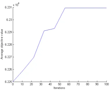
Figure 3 shows the convergence behavior of the proposed hybrid CP-SA algorithm when the iteration number ranges from 10 to 100 and the values for Pac0and Neare
[image:5.595.310.502.365.520.2]determined as 0.99 and 60, respectively.
Fig 3. Average objective values in different iterations
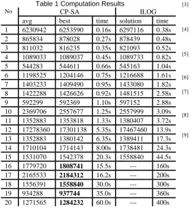
Table 1 summarizes the best and the average of the best solutions obtained by running the proposed hybrid algorithm 5 times. The average computation times needed to achieve the best solutions are also included.
Table 1 Computation Results
No CP-SA ILOG
avg best time solution time
1 6230942 6253590 0.16s 6297116 0.38s
2 865834 878028 0.27s 878439 0.48s
3 811032 816235 0.35s 821093 0.52s
4 1089033 1089037 0.45s 1089733 0.82s
5 544283 544611 0.66s 545163 1.04s
6 1198525 1204146 0.75s 1216688 1.61s 7 1403233 1409490 0.95s 1433080 1.82s 8 1422288 1426626 0.92s 1481515 2.58s
9 592299 592369 1.10s 597152 2.88s
10 2369706 2557677 1.25s 2557999 3.09s 11 1352883 1353818 1.33s 1380407 3.72s 12 17278360 17301138 5.35s 17467460 13.9s 13 1352883 1380142 6.35s 1389411 17.3s 14 1710104 1714143 8.00s 1738481 24.3s 15 1531070 1542378 20.3s 1558840 44.5s
16 1779720 1808741 15.5s --- 160s
17 2165533 2184312 16.2s --- 200s
18 1556391 1558840 30.0s --- 300s
19 934288 937744 35.0s --- 360s
20 1271565 1284232 60.0s --- 400s
V. CONCLUSIONS
In this paper, a novel mixed integer programming model has been formulated for solving the integrated supplier selection and order allocation problem that occurs in the design of a multi-product supply chain operating under a multi-period manufacturing scenario. A new hybrid CP-SA algorithm has also been developed by combining the strengths of both constraint programming and simulated annealing for solving this complex problem. In the hybrid algorithm, CP has been used to generate the initial feasible solution and SA has been used to guide the search path. Unlike traditional SA, CP has been used to generate the neighborhood solutions for SA. Useful information obtained from CP helps to reduce the search space. The proposed algorithm has been tested with a set of randomly generated test problems. Indeed, the proposed methodology has been shown to be efficient and effective for making optimal decisions on supplier selection and order allocation.
ACKNOWLEDGEMENT
The work described in this paper was supported by a grant from the research Grants Council of the Hong Kong Special Administrative Region, China (Project No. HKU 715409E).
REFERENCES
[1] Azizi, N., Zolfaghari, S., Adaptive temperature control for simulated annealing: a comparative study, Computers & Operations Research, 31, pp. 2439–2451, 2004.
[2] Bartak, R., “Theory and Practice of Constraint Propagation”, in
Proceedings of the 3rd Workshop on Constraint Programming for Decision and Control (CPDC2001), Wydavnictvo Pracovni Komputerowej, Gliwice, Poland, pp. 7-14, June 2001.
[3] C. Weber, J. Current, and W.Benton, “Vendor selection criteria and methods”, European Journal of Operational Research, Vol. 50, pp.2-18, 1991.
[4] C. Weber and J. Current, “A multi-objective approach to vendor selection”, European Journal of Operational Research, Vol. 68, pp.173-184, 1993.
[5] J. Jiao, “Generic bill-of-materials-and-operations for high variety production management”, Concurrent Engineering: Research and Application, Vol.8, No.4, pp.297-322, 2000.
[6] Kirkpatrick, S., Gelatt Jr., C.D., Vecchi, M.P., Optimization by simulated annealing. Science 1983, 220, pp. 671–680.
[7] L. Jacques, “An optimization model for selecting a product family and designing its supply chain”, European Journal of Operational Research, Vol. 169, pp.1030-1047, 2006.
[8] Tavakkoli-Moghaddam, R., Aryanezhad, M.B., Safaei, N., Azaron, A., Solving a dynamic cell formation problem using metaheuristics, Applied Mathematics and Computation, 170, pp.761-780,2005. [9] Tsang, E. Foundations of Constraint Satisfaction, Academic Press,