Abstract—Extreme maximum temperature using 10 years of
data is studied. Maximums of five different time periods (weekly, biweekly, monthly, quarterly and half yearly) are fitted to the Generalized Extreme Value (GEV) distribution. The results show that only weekly, biweekly, and monthly maximums are significant to be fitted to the GEV model and thus are used as our selection periods. Both the Augmented Dickey Fuller (ADF) and Kwiatkowski, Phillips, Schmidt and Shin (KPSS) stationarity tests detected no stochastic trends for maximum temperatures. However, the Mann-Kendall (MK) test shows that all three selection periods have a decreasing trend, suggesting that we ought to model for non-stationarity. Three models are considered and the model with a location parameter that increases with time is found to be the best for all selection periods. The Kolmogorov-Smirnov and Anderson-Darling goodness of fit tests show that all three selection period maximums converge to the GEV distribution with the weekly maximums having the best convergence to the GEV distribution. Estimates of the return level show that the return temperature which exceeds the maximum temperature of the observation period (35.6) starts to appear in the return period of T100 for monthly maximums, while for weekly and biweekly maximums, they are predicted to be more than 100.
Index Terms—Extreme, Maximum, Generalized Extreme
Value, Return Level
I. INTRODUCTION
XTREME Value Theory (EVT) differs from other typical statistical techniques in its objective to quantify the stochastic behaviour of a process at unusually large or small levels. It is based on the analysis of the maximum (or minimum) value in a selected time period. In general, EVT usually requires estimation of the probability of events that are more extreme than any that have already been observed.
Extreme value theory has been widely used and studied by many researchers. The earliest recorded application of extreme value was by astronomers in rejecting outlying
This work was supported in part by the Universiti Sains Malaysia under FRGS Grant 203/PMATHS/671123.
H. B. Hasan is with the School of Mathematical Sciences, Universiti Sains Malaysia, 11800 USM, Penang, Malaysia (phone: 604-653-3969; fax: 604-657-0910; e-mail: husna@ cs.usm.my, [email protected]).
N. B. Ahmad Radi is with Universiti Malaysia Pahang, Tun Razak Highway, 26300 Gambang, Pahang, Malaysia (e-mail: [email protected]).
S. B. Kassim is with the School of Mathematical Sciences, Universiti Sains Malaysia, 11800 USM, Penang, Malaysia (e-mail: ksuraya@
observations. Fuller [5] was probably the first to publish a paper that described an application of extreme values in flood flows. In 1920, Griffith applied extreme value theory to discuss the phenomena of rupture and flow in solids. Observations by Houghton et al. [12] show that daily minimum temperatures rise more significantly than daily maximum temperatures.
A. Background of Study
Humans are naturally captivated (both physically and intellectually) by the weather; it is a main topic of everyday conversations, while unusual or extreme weather events are major concerns as they can have enormous economic or human impact. Temperature extremes, which are attributed to an increasing concentration of greenhouse gases, are natural phenomena that affect our socio-economic activities. For example, extremely high temperatures and prolonged heat waves can damage agricultural production, increase energy and water consumption and also badly affect human well-being, human health and even cause loss of human lives (Karl and Easterling, [13]; Kunkel et al., [15]; Easterling et al., [4]). Thus, understanding and preparing for extreme weather events are essential for our society [3].
In this paper, our study focuses on extreme temperatures in Penang, an island off peninsular Malaysia. A study on extreme rainfalls has been done in [10]. Malaysia has an equatorial climate which means abundant sunshine, generally high heat, high humidity and high rainfall all year round. However, cloud cover cuts off a substantial amount of sunshine and on the average, Malaysia receives about 6 hours of sunshine per day. There are, however, seasonal and spatial variations in the amount of sunshine received. Being an island, the climate in Penang is very much influenced by the surrounding sea and the wind system. An increasing trend in the average surface temperature has been observed for Malaysia over the years. The western part of Malaysia where Penang island is located, was reported to experience more significant rise in temperature when compared to other regions in Malaysia and the months September-October-November recorded the highest temperature increase.
B. Objective of the study
Studies on extreme temperatures are beneficial to human understanding of extreme events. Decision-makers, risk management and researchers in climatology will benefit from knowledge about the behaviour of extreme
Modeling of Extreme Temperature Using
Generalized Extreme Value (GEV) Distribution:
A Case Study of Penang
Husna B. Hasan, Noor Fadhilah B. Ahmad Radi, and Suraiya B. Kassim
drawn to prepare the general public for changes due to extreme temperatures.
The objective of this study is to quantify and describe the behaviour of extreme temperature in Penang, Malaysia. In particular, we aim to model the extreme temperatures by using the Generalized Extreme Value (GEV) distribution. In the modeling process, we test for stationarity over different selection periods, namely, the weekly, biweekly, monthly, quarterly and half yearly periods. Next, we determine the best selection periods that are suitable for modeling with the GEV distribution by comparing their convergence to the GEV distribution. Lastly, we attempt to obtain the return level period that is expected to be exceeded.
C. Description of Data
The data which consists of daily temperatures measured (in Celcius) at the Bayan Lepas, Penang weather station, is obtained from the Malaysian Meteorological Department. The Bayan Lepas Regional Meteorological Office is the primary weather forecast facility for northern Peninsular Malaysia [22]. We consider the years 2000 to 2009 because this is the longest available period that is provided by the Malaysian Meteorological Services.
II. RESEARCH METHODOOGY
We consider Generalized Extreme value distributions having distribution functions of the form
Gmax( )y exp
[1 y]1
;
1y0 whereGmax( )y Pr(Yn y),
max
( ) / ( )
n n n n
Y M G y with Mn being the maximum selected among n values, as n , and is reduced with a location parameter nand a scale parameter,
n
, and is a shape parameter. This is the GEV family of distributions with the Frechet class of extreme value distribution corresponding respectively to the cases 0, while the Weibull distribution corresponds to 0 and the Gumbel distribution corresponds to 0 [1].
A. Selection Period
The GEV function provides a model for the distribution of block maxima. Its application consists of partitioning a data set into blocks of equal length, and fitting the GEV distribution to the set of block maxima. In implementing this model, the choice of block size has to be chosen so that individual block maxima has a common distribution. Temperature data are likely to have the same distribution as time increases. Inferences that fail to take this homogeneity into account would be likely to give inaccurate results. Normal considerations often lead to the adoption of blocks of length of one year. If a one year block is used, this study will only have 10 annual maximum temperature or 10 data points for the purpose of modeling, since we are using a 10-year data set; this is too few for any meaningful modeling. Thus, different selection periods are considered and compared; they are the weekly, biweekly, monthly, quarterly and half yearly block lengths.
B. Stationary Test
In order to fulfill the stationarity assumption of the generalized extreme value family of distributions, the Augmented Dickey Fuller (ADF) and Kwiatkowski, Phillips, Schmidt and Shin (KPSS) stationarity tests are performed on the data. The purpose of performing these two tests is to look for trends over different selection periods.
For the ADF test, the null hypothesis states difference stationarity while the alternative states stationarity. The null hypothesis of the KPSS test says that the distribution is stationary while the alternative says it is difference-stationary. The Mann-Kendall (MK) test which does not require normally distributed data and is well suited for analyzing datasets that have missing or tied data [6], is performed to detect the presence of monotonic trend (either increasing or decreasing). The null hypothesis states that no trend is present while the alternative states that there is a trend [19].
C. Model Choices and Parameter estimates
We look for the simplest model possible that explains as much of the variation in the data as possible. We consider three models; Model 1 is a basic model with constants µ, σ, and ξ, each referring to the location parameter, scale parameter and shape parameter, respectively. Model 2 is a four parameter model with µ being allowed to vary linearly with time, while other parameters are constants. Model 3 is a model where σ is an exponential function of time and other parameters are constants. The models are as follows:
Model 1: , , and constants
Model 2: ( )t 01t, , are constants
Model 3: ( )t exp(01t), , are constants
where the t’s are week units for weekly selection period, 2-weeks units for biweekly selection period, month units for monthly selection period, quarter units for quarterly selection period and half year units for half yearly selection period. For all models, the shape parameter, , is always a constant as this parameter is difficult to estimate with precision and it is usually unrealistic to try modeling as a smooth function of time.
The L-moments method (LMOM) is chosen as the parameter estimation technique for Model 1. The L-moments are expectations of certain linear combinations of order statistics and is a summary statistic for probability distributions and data samples. It is analogous to ordinary moments that provide measures of location, dispersion, skewness, kurtosis and other aspects of the shape of probability distributions or data samples. However, this method can only be used to estimate a stationary process; therefore, it is used to initialize the MLE routine for Model 1. This approach is not suitable for Models 2 and 3 because their parameters are functions of time; instead, the maximum likelihood estimation (MLE) method is used for Model 2 and Model 3.
D. Likelihood Ratio (LR) Test and Model Diagnostics Model 1 is compared to Model 2. Let L0 and L1be the
the four-parameter Model 2, respectively. The LR test statistic is defined as
0
1
2 log L L
and distributed as a chi-square distribution with one degree of freedom (corresponding to the difference in the number of parameters; in this case, 1). The three-parameter model is chosen if
1,0.952 3.8415.
Otherwise, the model with four parameters is preferred. Model 2 and Model 3 cannot be directly compared since they have the same number of parameters. Therefore, the result of Model 1 versus Model 2 will be compared with Model 3 since three models are considered in this study.
Various plots, such as the probability plot, quantile plot, return level plot and density plot are employed for diagnostics purposes. A quantile plot compares a model’s quantiles against the data (empirical) quantiles. A quantile plot that deviates greatly from a straight line suggests that the model assumptions may be invalid for the data plotted. The return level plot shows the return period against the return level, with an estimated 95% confidence interval. As useful as they are, graphical tests are not very accurate as compared to strong statistical tests, as pointed out by Lincoln [17]. Graphical tests are used more as a complement to the statistical analysis.
E. Kolmogorov-Smirnov and Anderson-Darling of Fit tests
The Kolmogorov-Smirnov and Anderson-Darling goodness of fit tests are used to assess the quality of convergence of the GEV distribution. The Kolmogorov-Smirnov test which is based on the empirical cumulative distribution function and the largest vertical difference between the theoretical and the empirical cumulative distribution function, is used to decide if a sample comes from a hypothesized continuous distribution. The Anderson-Darling procedure is a general test to compare the fit of an observed cumulative distribution function to an expected cumulative distribution function. This test gives more weight to the tails of a distribution than the Kolmogorov-Smirnov test. The null hypothesis of both tests is that the data follow the specified distribution.
F. Return level Estimate
A return level is the level that is expected to be exceeded on an average of once every t time periods. In this study, the return level is the maximum temperature amount and t corresponds to the selection intervals which are 1-week, 2
-weeks, a month, quarter year and half year. Return levels are important for prediction and planning purposes and can be estimated from stationary models.
III. FINDING AND DISCUSSIONS
A. Descriptive Statistics
The study involves 10 years of data consisting of daily maximum temperatures from year 2000 to 2009. Table 1 and Table 2 show the descriptive statistics for the daily
temperatures together with the various selection intervals. The maximum value is 35.6.
Table I and Table II show that the 3653 daily maximum temperatures has a standard deviation of 1.289 and quite a large coefficient of variation of 4.06, indicating a varied daily maximum temperature. After partitioning the data into different selection periods, it is observed that as the selection period increases, the difference between the minimum and maximum gets smaller, and the coefficient of variation decreases. This indicates that the maximum temperature data is less dispersed from the mean as the selection period increases.
TABLEI
SUMMARY STATISTICS OF MAXIMUM TEMPERATURE
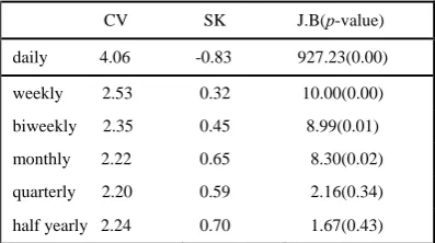
The skewness are positive for all selection periods although it is slightly negative on the daily temperature. This observation points to a distribution with a right tail which is relatively longer than the left tail. An increasing skewness indicates that the right tail becomes heavier as the selection period increases.
TABLEII
SUMMARY STATISTICS OF MAXIMUM TEMPERATURE
CV SK J.B(p-value)
daily 4.06 -0.83 927.23(0.00)
weekly 2.53 0.32 10.00(0.00)
biweekly 2.35 0.45 8.99(0.01)
monthly 2.22 0.65 8.30(0.02)
quarterly 2.20 0.59 2.16(0.34)
half yearly 2.24 0.70 1.67(0.43)
CV= Coefficient of Variation, SK = Skewness
The p-value of the Jarque-Bera (J.B) normality test, (which has a chi-squared distribution with two degrees of freedom) for the weekly, biweekly, and monthly maximum rejects the null hypothesis in favour of a non-normal distribution while the quarterly and half yearly maximums favour a normal distribution. Thus, the quarterly and half yearly periods are considered not appropriate. A check with the histogram of maximum temperature for the three selection periods (weekly, biweekly and monthly) supports right-skewed distributions. Therefore, we conclude that modeling with the GEV distribution with weekly, biweekly and monthly selection periods is reasonable for this study.
B. Testing for Stationarity
To check for the stationarity assumption, line graphs of the maximum temperatures are plotted for all selected intervals. The graphs show that there is no strong evidence of trends and no strong indication that the pattern of
N Min Mean S.Dev
Daily 3653 25.1 31.72 1.289
weekly 522 30.2 32.795 0.830
biweekly 261 31.3 33.102 0.777
monthly 120 32.2 33.408 0.743
quarterly 40 32.4 33.753 0.742
[image:3.595.318.517.433.544.2]variation in maximum temperatures has changed. This observation is supported by the Augmented Dickey Fuller (ADF) and Kwiatkowski, Phillips, Schmidt and Shin (KPSS) tests, as shown in Table III.
TABLEIII
UNIT ROOT TEST FOR MAXIMUM TEMPERATURE
Test critical value Test
SP test 1% 5% 10% Statistic
W
B
M
ADF KPSS
ADF KPSS
ADF KPSS
-3.980 0.216
-3.990 0.216
-4.040 0.216
-3.420 0.146
-3.430 0.146
-3.450 0.146
-3.130 0.119
-3.140 0.119
-3.150 0.119
-6.360 0.133
-5.430 0.121
-6.030 0.142 SP= Selection Period, W = weekly, B=biweekly, M = monthly
The p-values (0.00) of the ADF tests are significant at the 1%, 5% and 10% significance levels. The KPSS test shows that all the test statistics are insignificant at the 1% and 5% levels since all the test statistics have values which are smaller than the critical values over different selection periods. Hence, the null hypothesis cannot be rejected, favouring difference-stationarity. We therefore conclude that there is stationarity in maximum returns over the difference of selection periods at the 1% and 5% significance levels.
Performing the Mann-Kendall (MK) test under the null hypothesis of an absence of trends, we obtain the result as shown in Table IV below:
TABLEIV
MANN-KENDALL TEST
Selection Period
z
p-value
upward trend
downward trend weekly
biweekly monthly
-4.3426 -2.9861 -2.7193
0.9999 0.9986 0.9967
0 0 0
All three selection periods show the existence of a downward trend as time increases, contradicting the results of the stationary test. This results suggest that we ought to model for both stationarity and non-stationarity in this study.
C. Parameter Estimates and Model Selections
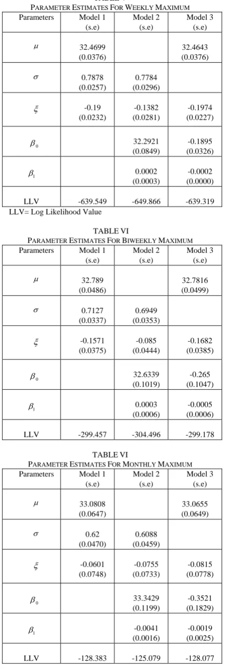
The parameter estimates over different selection periods for the three models considered in section II.C are shown in Table V to Table VII. Maximization of the GEV’s log-likelihood for weekly maximums leads to the parameter estimations for Model 1, Model 2, and Model 3, respectively and shown in Table V. The diagonal of the variance-covariance matrix of the parameter estimates corresponds to the variances of the individual parameters
( , , ) , with the standard errors listed in brackets.
Fitting the GEV distribution to the biweekly and monthly maximums leads to the maximum likelihood estimate as shown in Table VI and VII, respectively. It is noted that the
standard error (s.e) for all the parameters increase as the selection intervals increase.
TABLEV
PARAMETER ESTIMATES FOR WEEKLY MAXIMUM
Parameters Model 1
(s.e)
Model 2 (s.e)
Model 3 (s.e)
32.4699
(0.0376)
32.4643 (0.0376)
0.7878
(0.0257)
0.7784 (0.0296)
-0.19
(0.0232)
-0.1382 (0.0281)
-0.1974 (0.0227)
0 32.2921
(0.0849)
-0.1895 (0.0326)
1
0.0002
(0.0003)
-0.0002 (0.0000)
LLV -639.549 -649.866 -639.319
LLV= Log Likelihood Value
TABLEVI
PARAMETER ESTIMATES FOR BIWEEKLY MAXIMUM
Parameters Model 1
(s.e)
Model 2 (s.e)
Model 3 (s.e)
32.789
(0.0486)
32.7816 (0.0499)
0.7127
(0.0337)
0.6949 (0.0353)
-0.1571
(0.0375)
-0.085 (0.0444)
-0.1682 (0.0385)
0
32.6339 (0.1019)
-0.265 (0.1047)
1
0.0003
(0.0006)
-0.0005 (0.0006)
LLV -299.457 -304.496 -299.178
TABLEVI
PARAMETER ESTIMATES FOR MONTHLY MAXIMUM
Parameters Model 1
(s.e)
Model 2 (s.e)
Model 3 (s.e)
33.0808
(0.0647)
33.0655 (0.0649)
0.62
(0.0470)
0.6088 (0.0459)
-0.0601
(0.0748)
-0.0755 (0.0733)
-0.0815 (0.0778)
0
33.3429 (0.1199)
-0.3521 (0.1829)
1
-0.0041
(0.0016)
-0.0019 (0.0025)
[image:4.595.316.543.82.754.2] [image:4.595.55.291.439.517.2]The likelihood-ratio test is used to compare the three models and the test statistic and p-values are listed in Table VIII and Table IX.
TABLEVIII
MODEL 1 VS MODEL 2
Model 1 vs Model 2 p-value
weekly biweekly monthly 6.6071 10.0775 20.6351 0.0102 0.0015 0.0000 TABLEIX
MODEL 1 VS MODEL 3
Model 1 vs Model 3 p-value
weekly biweekly monthly 0.6104 0.5575 0.4592 0.4346 0.4553 0.4979
Comparing Model 1 with Model 2 (Table VIII), we observe that Model 2 is a slight improvement from Model 1 over different selection intervals. From Table 9, Model 1 is preferred over Model 3 for all selection periods.
Since Model 1 is better than Model 3, while Model 2 is better than Model 1, we can therefore conclude that Model 2, where is allowed to vary linearly with respect to time, and other parameters are constants, is the best among the three models over different selection periodss. This result is also supported by an earlier Mann-Kendal test which concluded that there exists a downward trend as time increases.
D. Model Diagnostics
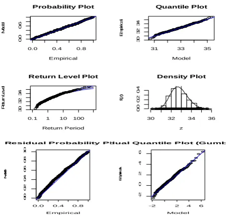
Figure 1(a) and 1(b) shows the model diagnostics for weekly maximums for Model 1, Model 2 and Model 3, respectively. Inspection of Model 1 diagnostics shows that neither the probability plot nor the quantile plot doubt the validity of the fitted model since each set of plotted points appears to be linear. The return level plot shows approximate linearity, since is close to zero.
0.0 0.4 0.8
0. 0 0. 6 Probability Plot Empirical M odel
31 33 35
30 3 2 34 Quantile Plot Model E m pi ri c al 30 32 34 Return Period R et u rn Lev e l
0.1 1 10 100
Return Level Plot Density Plot
z
f(
z
)
30 32 34 36
0. 0 0. 2 0. 4
0.0 0.4 0.8
0 .0 0 .2 0 .4 0 .6 0 .8 1 .0 Empirical M o d e l
Residual Probability Pl
-2 2 4 6
-2 0 2 4 6 Model E m p ir ic a l
dual Quantile Plot (Gumb
Fig. 1(a): Model Diagnostic for Weekly Maximum
0.0 0.4 0.8
0 .0 0 .2 0 .4 0 .6 0 .8 1 .0 Empirical M o d e l
Residual Probability Pl
-2 2 4 6
-2 024 6 Model E m p ir ic a l
dual Quantile Plot (Gumb
Fig. 1(b): Model Diagnostic for Weekly Maximum
For Model 2 and Model 3, only the residual probability and quantile plots are displayed with the quantile plot on the Gumbel scale. All plots suggest that all models have a good fit. Inspection on biweekly and monthly maximum (not shown here) resulted in similar results.
E. Kolmogorov-Smirnov and Anderson-Darling of Fit Test
Table X shows the Kolmogorov-Smirnov and Anderson-Darling test results over different selection periods. Modeling using the different selection periods resulted in almost similar fits. An inspection of the p-values leads to a non-rejection of the null hypotheses over the different selection periods. However, as the selection period increases, convergence to the GEV is most likely to be better for the weekly selection period as its p-value is smaller than the p-values for the other two selection periods.
TABLEX
KOLMOGOROV-SMIRNOV (KS) AND ANDERSON-DARLING (AD)
sample size statistics p-value
(weekly=522) KS AD 0.04275 0.6332 0.28751 -(biweekly=261) KS AD 0.05437 0.48604 0.40872 - (monthly = 120)
KS AD 0.06093 0.33153 0.74108
-Thus, we further conclude that the data follow the specified distribution for weekly, biweekly and monthly selection periods. An inspection of the graphs of the p.d.f. of a GEV distribution revealed that weekly maximums show better convergence to the GEV distribution than the other two selection periods.
F. Return Level Estimate
The highest daily temperature for the 10-year observation period is 35.6. To predict the probability that a daily maximum temperature exceeding 35.6 will occur in a longer period, return levels are used. The return levels are estimated by using Model 1 (stationary) of weekly, biweekly and monthly maximums.
[image:5.595.322.536.54.142.2] [image:5.595.61.288.87.220.2] [image:5.595.61.291.507.728.2]TABLEXI(A)
RETURN LEVEL ESTIMATE FOR T5, 10 Selection
period T5 T10
weekly 33.498
(33.409, 33.5910)
33.9123 (33.8115, 34.0231)
biweekly 33.7413
(33.6223, 33.869)
34.1398 (34.0022, 34.3016)
monthly 33.9701
(33.7961,34.172)
34.3859 (34.1717, 34.6901)
TABLEXI(B)
RETURN LEVEL ESTIMATE FOR T50, 100 Selection
period T50 T100
weekly 34.6404
(34.4977, 34.8286)
34.8858 (34.7192, 35.1185
biweekly 34.8677
(34.6601, 35.1804)
35.123 (34.8745, 35.5229 )
monthly 35.2375
(34.8512, 36.0238)
35.5729 (35.0792,36.6318)*
The table also shows that the temperature which exceeds the maximum temperature (35.6) of the observation period appears in the confidence interval of T100 for monthly maximums. For weekly and biweekly maximums, the temperature which exceeds the maximum temperature (35.6) of the observation period is predicted to occur in more than T 100.
IV. SUMMARY AND CONCLUSION
Generalized Extreme Value (GEV) distribution is used to model maximum temperatures using data obtained from Penang weather station for the period from 2000 to 2009. Stationarity tests shows that all the selection periods are stationary while a trend test revealed a decreasing trend.
All selection periods are fitted to the GEV distribution and the parameters are estimated. The likelihood ratio test suggests that the best model is a model with a location parameter that increases linearly with time, and the scale and shape parameters are constants. Model diagnostics which include probability plot, quantile plot, return level plot and density plot show a good fit. The Kolmogorov
-Smirnov and Anderson-Darling goodness of fit tests show that modeling using the different selection periods resulted in almost similar fits. However, modeling using weekly maximum gave the best convergence to the GEV distribution.
The return level estimate, which is the return level that is expected to be exceeded in a certain period of time is estimated at T5, 10, 50 and 100. The results revealed that the temperature which exceeds the maximum temperature amount (35.6) of the observation period starts to appear in the confidence interval of T100 for monthly maximums. For weekly and biweekly maximum, the temperature which exceeds the maximum temperature
(35.6) of the observation period is predicted to be more than the period for this study.
In conclusion, modeling maximum temperatures using GEV distribution seems reasonable even though only 10 years of data are available.
ACKNOWLEDGMENT
The authors would like to thank the Bayan Lepas Regional Meterological Office for providing the data.
REFERENCES
[1] T. G. Bali, . The generalized extreme value distribution. Economics
letters 79, 423-427, 2003.
[2] S. Coles,. An Introduction to Statistical Modelling of Extreme Values.
Great Britain: Springer, 2001.
[3] D. S. Cooley, Statistical Analysis of Extremes Motivated by Weather
and Climate Studies: Applied and Theoretical Advances. PhD theses, University of Colorado, 2005.
[4] D. R Easterling, J. L. Evans, P. Y. Groisman, T. R. Karl, K. E.
Kunkel, P. Ambenje,, Observed variability and trends in extreme
climate events. Bulletin of American Meteorological Society 81, 417–
425, 2000.
[5] W. E. Fuller, Flood Flows, Transactions of the American Society of
Civil Engineers. 77, 564, 1914.
[6] R. O. Gilbert, Statistical methods for environmental pollution
monitoring. New York: Van Nostrand Reinhold, 1987.
[7] A. A. Griffith, The Phenomena of Rupture and Flow in Solids.
Philosophical Transactions of the Royal Society of London. 221, 163– 98, 1920.
[8] E. J. Gumbel, The Return Period of Flood Flows. Annals of
Mathematical Statistics. 12, 163–90, 1941.
[9] E. J. Gumbel, Floods Estimated by Probability Methods. Engineering
Record. 134, 97News—101, 1945.
[10] H. Hasan, W. C. Yeong, Extreme Value Modeling and Prediction of
Exterme Rainfall: A Case Study of Penang, AIP Conf. Proc, V1309,
p372-393.
[11] H. Hasan, N. F. Ahmad Radi, S. Kassim, Modeling the Distribution
of Extreme Share Return in Malaysia Using Generalized Extreme
Value (GEV) Distribution, AIP Conf. Proc, V1450, to be published.
[12] J. T. Houghton, Y. Ding, D. J. Griggs, M. Noguer, M.,P. J. van der
Linden, D. Xiaosu, In: IPCC Third Assessment Report: Climate
Change 2001: The Scientific Basis. Cambridge University Press, Cambridge, pp. 944, 2001.
[13] T. R. Karl, D. R. Easterling, Climate extremes: selected review and
future research directions. Climatic Change 42, 309–325, 1999.
[14] S. Kotz, S. Nadarajah, Extreme Value Distributions, Theory and
Applications (Imperial College Press), 1999.
[15] K. E. Kunkel, R. A. Pritke, S. A. Changnon, Temporal fluctuation in
weather and climate extremes that cause economic and human health
impacts—a review. Bulletin of American Meteorological Society 80,
1077–1098, 1999
[16] F. M. Longin, The asymptotic distribution of extreme stock market
returns.The Journal of Business, 69 (3), 383-408, 1996
[17] E. M. Lincoln, Graphical Methods in Statistical Analysis. Annual
Reviews Public Health. 8, 309-353, 1987.
[18] National Environment Agency (2002). The Climate of Malaysia
[Online], [Accessed 2nd August 2011]. Available from World Wide Web: http://app2.nea.gov.sg/asiacities_malaysia.aspx
[19] S. Winkler, Technical Publication Sj2004-4: A User-Written SAS
Program for Estimating Temporal Trends and Their Magnitude. Palatka, Florida: St. John Water Management, 2004.
[20] E. Zivot, J. Wang, Modelling Financial Time Series with S-Plus.
United States of America: Springer, 2006.
[21] Wikipedia (2011). Penang [Online], [Accessed 2nd August 2011].
Available from the World Wide Web: http://en.wikipedia.org/wiki/Penang