Notes for Discrete-Time Control Systems (ECE-420) Fall 2013

(1)

Notes for Discrete-Time Control Systems

(ECE-420)

Fall 2013

by R. Throne The major sources for these notes are

• Modern Control Systems, by Brogan, Prentice-Hall, 1991.

• Discrete-Time Control Systems, by Ogata. Prentice-Hall, 1995.

• Computer Controlled Systems, by ˚Astr¨om and Wittenmark. Prentice-Hall, 1997.

• Analog and Digital Control System Design, by C. T. Chen. Sanders College Publishing. 1993.

• Digital Control of Dynamic Systems, by Franklin, Powell, and Workman. Addison Wesley, 1998.

(2)

-Transforms

In this course we will assume we are sampling the continuous time signal x(t) at a uniform sampling rate. The time interval between samples will be denoted by T. Thus we will denote the discrete-time (sampled) values as x(0), x(T), x(2T),. . ., x(kT). This is shown graphically in Figure 1. Sometimes we remove the explicit dependence on the sampling interval T and just write x(0), x(1), x(2), . . . , x(k), since the sample interval is the same for all of the diﬀerent samples.

1.1

Special Functions

Just as in continuous-time, there are certain special functions that are used very often in discrete-time. Speciﬁcally, we will be concerned with the unit impulse function, the unit step function, and the unit ramp function.

The unit impulse ordelta function is deﬁned as δ(k) =

1 k = 0 0 k = 0 or

δ(n−k) =

1 k−n= 0 0 k−n= 0 The unit step orHeaviside function is deﬁned as

u(k) =

1 k≥0 0 k <0 or

u(n−k) =

1 n−k ≥0 0 n−k < 0 The unit rampfunction is deﬁned as

r(k) = ku(k) or

r(n−k) = (n−k)u(n−k)

While there are other special function, these are the special functions we will be utilizing the most.

1.2

Impulse Response and Convolution

The unit impulse response of a Linear Time-Invariant (LTI) system, h(k), is the response of the system at rest (no initial energy, the initial conditions are all zero), to a unit impulse at time zero. Symbolically, we can write

δ(k)→h(k)

(5)

x(t)

0

x(0)

T x(T)

2T

x(2T)

3T

x(3T)

4T

x(4T)

5T

x(5T)

6T

Figure 1: Continuous-time signalx(t) and its samplesx(kT). We assume the samples are taken at the beginning of each time interval.

Since the system is also linear, we have

αδ(k)→αh(k) and

αδ(n−k)→αh(n−k) Now we can write x(n) as

x(n) =. . .+x(−2)δ(n+ 2) +x(−1)δ(n+ 1) +x(0)δ(n) +x(1)δ(n−1) +x(2)δ(n−2) +. . . If x(n) is the input to an LTI system, then we can compute the output as

y(n) =. . .+x(−2)h(n+ 2) +x(−1)h(n+ 1) +x(0)h(n) +x(1)h(n−1) +x(2)h(n−2) +. . . since we treat the x(k)’s as constants, and the system is only responding the the impulses. We can write this expression as

y(n) =

∞

k=−∞

x(k)h(n−k)

or, by making a change of variable in the sum, as y(n) =

∞

k=−∞

(6)

Thus the output of an LTI system is the convolution of the input with the impulse response of the system,

y(n) = h(n) x(n) =

∞

k=−∞

h(k)x(n−k)

= x(n) h(n) =

∞

k=−∞

x(k)h(n−k)

If both the system and input are causal (both are zero for n ≤ 0), then we can simplify the convolution sums as

y(n) = h(n) x(n) =

n

k=0

h(k)x(n−k)

= x(n) h(n) =

n

k=0

x(k)h(n−k)

1.3

A Useful Summation

In what follows, we will make extensive use of a simple summation formula, which you probably saw in high school. Let’s denote the sum Sn as

Sn = 1 +a+a2+. . .+an−1+an= k=n k=0

ak

If we multiply by a we have

aSn = a

1 +a+a2+. . .+an−1+an = a+a2+a3+. . .+an+an+1 = Sn−1 +an+1

Solving for Sn we have

aSn−Sn = an+1−1

Sn =

an+1−1 a−1 or

k=n k=0

ak = 1−a

n+1

1−a Note that if n=∞ and |a|<1, then we have

∞

k=0

(7)

Example.Assume the input to a system isx(n) =u(n) and the impulse response of the system is h(n) =u(n). Determine the output of the system. We have

y(n) = x(k) h(k) =

∞

k=−∞

x(k)h(n−k)

=

k=−∞

u(k)u(n−k)

=

n

k=0

(1)(1) = (n+ 1)u(n)

Note that we need the ﬁnal u(n) since our method is only valid if n ≥0.

Example. Assume the input to a system is x(n) =αnu(n) and the impulse response is h(n) = u(n). Determine the output of the system. We have

y(n) = x(k) h(k) =

∞

k=−∞

x(k)h(n−k)

=

k=−∞

αku(k)u(n−k)

=

n

k=0

αk

= 1−α

n+1

1−α u(n)

Note that we need the ﬁnal u(n) since our method is only valid if n ≥0.

Example. Assume the input to a system is x(n) = αn+2_u(n_{+ 2) and the impulse response is}

h(n) = βn−1_u(n₋_{1). Determine the output of the system. We have}

y(n) = x(k) h(k) =

∞

k=−∞

x(k)h(n−k)

=

k=−∞

αk+2u(k+ 2)βn−k−1u(n−k−1)

Now let’s look at our sums. We know u(k + 2) = 1 for k ≥ −2 and u(n −k −1) = 1 for n−k−1≥0 or n−1≥k. Hence our sum is

y(n) =

n−1 k=−2

αk+2βn−k−1

In order to use our summation formula, let’s change variables in this sum. We want the lower limit to be zero, so let’s deﬁne l=k+ 2, ork =l−2. In terms ofl, our new sum is

y(n) =

l=n+1 l=0

(8)

= βn+1

n+1 l=0

α β

l

= βn+1 ⎡ ⎣1−(

α β)

n+2

1− α β

⎤

⎦u(n+ 1)

Example. Assume the input to a system is x(n) = α−n_u(−_{n) and the impulse response is}

h(n) = βn−1_u(n₋_{1). Determine the output of the system. We have}

y(n) = x(k) h(k) =

∞

k=−∞

x(k)h(n−k)

=

k=−∞

α−ku(−k)βn−k−1u(n−k−1)

We know thatu(−k) = 1 fork ≤0 andu(n−k−1) = 1 forn−k−1≥0 ork ≤n−1. Now we have to be very careful since our answers will depend on what we assume about n. For n ≥1, the most restrictive condition is k ≤0 Our new sum becomes

y(n) =

0

k=−∞

α−kβn−k−1

= βn−1

0

k=−∞

(αβ)−k

Letting l = −k and assuming the sum is absolutely convergent so that we can rearrange the order of the summation, we have

y(n) = βn−1

l=∞ l=0

(αβ)l =βn−1 1 1−αβ

Next, let’s look at what happens for n ≤ 0. Here the more restrictive condition is k ≤ n−1, and we have the sum

y(n) =

n−1 k=−∞

α−kβn−k−1

= βn−1

n−1 k=−∞

(αβ)−k Letting l=k−(n−1) =k−n+ 1 we have

y(n) = βn−1(αβ)−(n−1)

0

l=−∞

(αβ)−l Finally, let p=−l and assume absolute convergence, and we have

y(n) = α−n+1 1 1−αβ Combining our two regions we have

y(n) = βn−1 1

1−αβu(n−1) +α

−n+1 1

(9)

1.4

z

-Transforms

In continuous-time we can either compute the output of a system using the convolution directly, or we can resort to transform methods. In continuous-time control systems we generally utilize Laplace transforms and block diagrams, since this is a much easier way to determine the output than by using convolution in the time domain. Similarly, in discrete-time we can utilize the z-transform to avoid using the convolution sum. Just as with Laplace transforms, we can deﬁne one and two-sided z-transforms.

The one-sided z-transform is deﬁned as

X(z) = Z {x(nT)}=

∞

k=0

x(kT)z−k

and the two-sided z-transform is deﬁned as

X(z) = Z {x(nT)}=

∞

k=−∞

x(kT)z−k

Just as with Laplace transforms, the only diﬀerence between the one and two-sidedz-transform is the lower limit. Often we do not directly utilize the dependence on T and leave it out of the summation. In this course we are generally concerned with causal systems and causal inputs, so we generally will use the one-sided z-transform. Finally, the sum often only converges for values of |z| within a speciﬁc region. This is called the region of convergenceorROC. Now let’s do some examples.

Example. Determine the one-sided z-transform ofx(n) =δ(n−l). We have

X(z) =

k=∞ k=0

δ(k−l)z−k =z−l

This sum converges for all values of|z|, so the region of convergence is the entire z-plane. Example. Determine the one-sided z-transform of x(n) = u(n), the unit step function. We have

X(z) =

∞

k=0

u(k)z−k=

∞

k=0

₁ z

k

= 1

1−z−1 = z z−1

This is only true if the sum is absolutely convergent, which means |1_z|<1 or if |z| >1. Hence the ROC is deﬁned by |z|>1.

Example. Determine the one-sided z-transform of x(n) = nu(n), the unit ramp function. We have

X(z) =

∞

k=0

ku(k)z−k=

∞

k=0

(10)

At this point, we need to use something we all ready know, and some calculus. For the unit step we have

z z−1 =

∞

k=0

z−k

Taking derivatives of both sides with respect to z yields d

dz _z

z−1

= (z−1)−z (z−1)2 =

−1 (z−1)2 d

dz _∞

k=0

z−k

=

∞

k=0

−kz−k−1 =−z−1

∞

k=0

kz−k

Hence we have

−1

(z−1)2 = −z

−1∞

k=0

kz−k or

∞

k=0

kz−k = z (1−z)2

which is the result we wanted. Just as with the z-transform of the unit step, the ROC for this function is|z|>1.

Example. Determine the one-sided z-transform for the function x(n) =anu(n). We have X(z) =

∞

k=−∞

aku(k)z−k

=

∞

k=0

_a z

k

= 1

1−a_z = z z−a The region of convergence is given by |a

z|<1 or |z|>|a|.

Example.Determine thez-transform of thex(t) =e−atu(t) whenx(t) is sampled with sampling interval T. The sampled version of the signal is given by x(nT) =e−anT_u(nT_{) =}_e−aTn_u(n).

Computing the z-transform we have X(z) =

∞

k=−∞

e−aTku(k)z−k

=

∞

k=0

₁ eaT_z

k

= 1

1− _e_aT1_z

= z

(11)

The region of convergence is given by |_eaT1_z|<1 or e−aT <|z|.

Example. Find the one-sided z-transform of x(n) =ancos(bnT)u(n). We have X(z) =

∞

k=−∞

akcos(bkT)u(k)z−k =

∞

k=0

a z

k

cos(bkT) At this point we need to use Euler’s identity,

cos(bkT) = e

jbkT ₊_e−jbkT

2 =

1 2

ejbTk+1 2

e−jbTk Inserting this identity into our sum we have

X(z) = 1 2

∞

k=0

_a ze

jbT

k

+ 1 2

∞

k=0

_a ze

−jbT

k

= 1 2

1 1− aejbT_z +

1 2

1 1− ae−_zjbT After some algebra we arrive at

X(z) = z(z−acos(bT)) z2−2acos(bT)z+a2 the region of convergence is given by

|aejbT

z |<1, | ae−jbT

z |<1 or|z|>|a| since |ejbT|=|e−jbT|= 1.

1.5

z

-Transform Properties

Just as with Laplace and Fourier transforms, there are a number of useful properties of z-transforms. We will cover a few of them in this section. Most of the properties we will cover are straightforward to prove, and you should be able to prove most of them. Unless otherwise stated, we will assume only one-sided z transforms.

Linearity. If we have the z-transform pairs g(n) ↔ G(z) and h(n) ↔ H(z), then for all constants a and b we have

Z {ag(n) +bh(n)} =aG(z) +bH(z) Multiplication by an. If g(n)↔G(z), thenang(n)↔G(_az).

Proof:

Z {ang(n)} =

∞

k=0

akg(k)z−k

=

∞

k=0

g(k) _z

a ₋k

(12)

Shifting. If g(n)↔G(z) and g(n) is causal, then

Z {g(n−l)} = z−lG(z)

Z {g(n+l)} = zl

G(z)−

l−1

k=0

g(k)z−k

Proof of ﬁrst part: Taking thez-transforms we have

Z {g(n−l)} =

∞

k=0

g(k−l)z−k

=

∞

k=l

g(k−l)z−k

since g(n) is causal. Now let m=k−l, or k =m+l. The sum then becomes

Z {g(n−l)} =

∞

m=0

g(m)z−(m+l)

= z−l

∞

m−0

g(m)z−m = z−lG(z)

Proof of the second part: Let’s start by trying to ﬁnd the z-transform of g(n+ 1). We have then

Z {g(n+ 1)} =

∞

k=0

g(k+ 1)z−k

= g(1) +g(2)z−1+g(3)z−2+g(4)z−3+g(5)z−4+. . .

Now we know G(z) =

∞

k=0

g(k)z−k

= g(0) +g(1)z−1+g(2)z−2+g(3)z−3+g(4)z−4+g(5)z−5+. . . Rearranging this expression we get

zG(z) = g(0)z+g(1) +g(2)z−1+g(3)z−2+g(4)z−3+g(5)z−4+. . . zG(z)−g(0) = g(1) +g(2)z−1+g(3)z−2+g(4)z−3+g(5)z−4+. . .

= Z {g(n+ 1)}

Now consider taking the z-transform of g(n+ 2). We have

Z {g(n+ 2)} =

∞

k=0

g(k+ 2)z−k

(13)

Starting from the deﬁnition of G(z) from above

G(z) = g(0) +g(1)z−1+g(2)z−2+g(3)z−3+g(4)z−4+g(5)z−5+. . . we can ﬁnd

z2G(z) = g(0)z2+g(1)z+g(2) +g(3)z−1+g(4)z−2+g(5)z−3+. . . z2G(z)−z2g(0)−zg(1) = g(2) +g(3)z−1+g(4)z−2 +g(5)z−3+. . .

= Z {g(n+ 2)} In general we have

Z {g(n+l)} =

∞

k=0

g(k+l)z−k

= g(l) +g(l+ 1)z−1+g(l+ 2)z−2+g(l+ 3)z−3+. . . and

G(z) = g(0) +g(1)z−1+g(2)z−2+. . .+g(l−1)zl−1+g(l)z−l+g(l+ 1)z−l−1+g(l+ 2)z−l−2+. . . zlG(z) = zlg(0) +zl−1g(1) +zl−2g(2) +. . .+z−1g(l−1) +g(l) +g(l+ 1)z−1+g(l+ 2)z−2+. . .

Rearranging we get

zlG(z)−zlg(0)−zl−1g(1) +zl−2g(2) +. . .+z−1g(l−1) = g(l) +g(l+ 1)z−1+g(l+ 2)z−2 +. . . zl

G(z)−

l−1

k=0

g(k)z−k

= Z {g(n+l)}

Final Value Theorem. Just as with Laplace transforms, the Final Value Theorem is very useful for determining steady state errors in discrete-time control systems. If we assume g(k) is causal, and all poles of G(z) are inside the unit circle (with exception of a possible simple pole atz = 1), then

lim

t→∞x(t) = limz→1

1−z−1G(z) = lim

z→1

z−1 z G(z)

Example. If g(t) = (1−e−3t_{)u(t), then} _{G(z) =} z(1−e−3T)

(z−1)(z−e−3T). By the Final Value Theorem we

have

lim

t→∞g(t) = 1 = limz→1

z−1

z G(z) =

1−e−3T

1−e−3T = 1

since all of the poles of the system are within the unit circle with the exception of a simple pole atz = 0.

Example. If g(t) =e−t_{u(t), then} _{G(z) =} z

z−e−T. By the Final Value Theorem

lim

t→∞g(t) = 0 = limz→1

z−1

(14)

since all of the poles of the system are within the unit circle.

Example. If g(t) =u(t), then G(z) = _z₋z₁. By the Final Value Theorem lim

t→∞g(t) = 1 = limz→1

z−1

z G(z) = 1 Note that in this example there is a simple pole at z = 1.

Initial Value Theorem. Just as with laplace transforms, the Initial Value Theorem for z-transforms is very useful for determining the initial required control eﬀort for diﬀerent types of controllers. The Initial Value Theorem states that if the limits exist, then

lim

t→0g(t) = limz→∞G(z)

Example. Ifg(t) = (1−e−3t_{)u(t), then} _{G(z) =} z(1−e−3T)

(z−1)(z−e−3T). By the Initial Value Theorem we

have

lim

t→0g(t) = 0 = limz→∞G(z) = 0

Example. If g(t) =e−t_{u(t), then} _{G(z) =} z

z−e−T. By the Initial Value Theorem

lim

t→0g(t) = 1 = limz→∞G(z) = 1

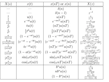
Table 1 summarizes some common z-transform pairs, while Table 2 summarizes some common z-transform properties.

1.6

Inverse

z

-Transforms

There are four common methods for going from thez-domain back to the (discrete) time domain. These are

• Computational methods (Matlab/Maple, etc)

• Contour integration in the complex plane

• Partial fractions

• Long division

In this course we will emphasize the use of partial fractions, which you should be pretty familiar with. It is generally easiest to ﬁnd the partial fraction expansion for G(_zz) when you want to ﬁnd the inverse z-transform of G(z), since simple poles have the form aku(k)↔ _z₋z_a.

Example. Determine g(n) forG(z) = ₍_z₋z(₃₎₍z−_z4)₋₂₎. We have G(z)

z =

z−4

(z−3)(z−2) = A z−3+

(15)

X(s) x(t) x(nT) or x(n) X(z)

— — δ(n) 1

— — δ(n−l) z−l

1

s u(t) u(nT)

z z−1

1

s+a e−

at_u(t) _e−anT_u(nT₎ z

z−e−aT

1

s2 tu(t) (nT)u(nT)

T z

(z−1)2

1

s3

1

2t2u(t) 12(nT)2u(nT)

T2z(z+1)

(z−1)3 a

s(s+a) (1−e−

at_)u(t) ₍₁₋_e−anT_)u(nT₎ z(1−e−aT)

(z−1)(z−e−aT) b−a

(s+a)(s+b) (e−

at₋_e−bt_)u(t) _(e−anT ₋_e−bnT_)u(nT₎ z(e−aT−e−bT)

(z−e−aT)(z−e−bT)

1

(s+a)2 te−

at_u(t) _(nT_)e−anT_u(nT₎ zT e−aT

(z−e−aT)2 s

(s+a)2 (1−at)e−

at_u(t) ₍₁₋_anT_)e−anT_u(nT₎ z[z−(1+aT)e−aT]

(z−e−aT)2 ω

s2+ω2 sin(ωt)u(t) sin(ωnT)u(nT)

zsin(ωT) z2−2zcos(ωT)+1 s

s2+ω2 cos(ωt)u(t) cos(ωnT)u(nT)

z[z−cos(ωT)] z2−2 cos(ωT)+1

bnu(n) _z₋z_b

nbn_u(n) bz

(z−b)2

(1−bn_)u(n) z(1−b)

(z−1)(z−b)

Table 1: Common (one sided) z-transforms. Often we set T = 1 and e−aT ₌ _b _{to ﬁnd results}

when the sampling time is not important.

x(t) x(nT) Z[x(t)] or Z[x(nT)]

αx(t) αx(nT) αX(z)

αx₁(t) +βx₂(t) αx₁(nT) +βx₂(nT) αX₁(z) +βX₂(z)

x(t+T) x(nT +T) zX(z)−zx(0)

x(t+ 2T) x(nT + 2T) z2X(z)−z2x(0)−zx(T)

x(t+kT) x(nT +kT) zk_X(z)−_zk_x(0)−_zk−1_x(T₎−_zk−2_X(2T₎−_{. . .}−_zx(kT −_T₎

x(t−kT) x(nT −kT) z−kX(z)

tx(t) (nT)x(nT) −T z_dzdX(z)

e−at_x(t) _e−anT_x(nT₎ _X(zeaT₎

— anx(nT) X(z_a)

x(0) x(0) limz→∞X(z) if the limit exists

x(∞) x(∞) limz→1[(1−z−1]X(z) if all poles ofX(z) are inside unit

the unit circle (a simple pole at z = 1 is allowed)

— n_k₌₀x(k) z

z−1X(z)

[image:15.612.122.505.91.377.2]

x(t) h(t) x(nT) h(nT) X(z)H(z)

Table 2: Common properties of (one sided) z-transforms. Often we set T = 1 and e−aT ₌_b _to

(16)

Using the ”cover up” method we quickly arrive at A= 3−4

3−2 =−1 B = 2−4 2−3 = 2 This leads to

G(z)

z =

−1 z−3+

2 z−2 or

G(z) =− z z−3+ 2

z z−2 From this form we can quickly conclude that

g(n) = −(3)nu(n) + 2(2)nu(n)

The ﬁrst few terms of this impulse response areg(0) = 1,g(1) = 1,g(2) =−1, andg(3) =−11. Example.Determine g(n) if G(z) = z−4

(z−3)(z−2). For thisG(z), there is no z in the numerator to

divide by to create the G(_zz). One solution is to multiple by z_z and then do the partial fractions, as follows:

G(z) = z−4

(z−3)(z−2) =

z−4 (z−3)(z−2)

z z so we have

G(z)

z =

z−4

z(z−3)(z−2) = A

z + B z−3+

C z−2 Using the ”cover up” method we get

A = −4

(−3)(−2) =

−2

3 , B =

3−4 (3−2)(3) =

−1

3 , C =

2−4

(2−3)(2) = 1 so

G(z) =−2 3−

1 3

z z−3 +

z z−2 which yields

g(n) =−2

3δ(n)− 1 3(3)

n_{u(n) + (2)}n_u(n)

If we compute the ﬁrst few terms of g(n) we get g(0) = 0, g(1) = 1, g(2) = 1, g(3) = −1, g(4) =−11.

Example. Determine g(n) if G(z) = ₍_z₋z₃₎₍−4_z₋₂₎. For this G(z), there is no z in the numerator to divide by to create the G(_zz). One solution is to construct andF(z) so that G(z) =z−1F(z) , as follows:

F(z) = z(z−4) (z−3)(z−2) so we have

F(z)

z =

z−4

(z−3)(z−2) = A z−3+

(17)

Using the ”cover up” method we get

F(z) =− z z−3+ 2

z z−2 and

f(n) =−(3)nu(n) + 2(2)nu(n)

Since we know G(z) =z−1F(z), we have g(n) =f(n−1) using the delay property. Hence g(n) = −(3)n−1u(n−1) + 2(2)n−1u(n−1)

Although this answer looks much diﬀerent than in the previous example, the two solutions are in fact the same.

Example. Determine g(n) forG(z) = ₍z_z(₊₁₎₍−5z_z+22)₋₂₎2. We have G(z)

z =

−5z+ 22 (z+ 1)(z−2)2 =

A z+ 1 +

B z−2 +

C (z−2)2 Using the ”cover-up” method we can quickly ﬁnd A and C,

A= −5(−1) + 22 (−1−2)2 =

27

9 = 3, C =

−5(2) + 22 (2 + 1) =

12 3 = 4

To get B, we multiply both sides of the original equation by z and then let z → ∞, to get 0 =A+B, B =−3

So we have

G(z) = 3 z z+ 1 −3

z z−2+ 4

z (z−2)2 and

g(n) = 3(−1)nu(n)−3(2)nu(n) + 4n(2)n−1u(n)

The ﬁrst few terms of the impulse response are g(0) = 0, g(1) = −5, g(2) = 7, g(3) = 21, and g(4) = 83.

While we can normally use partial fractions to determine the time response for all sample times, sometimes we only want to determine the time response for the ﬁrst few terms. We can use the method of long division to determine the ﬁrst few terms of the time domain response by utilizing the fact that if we compute the z-transform of g(n) we have

G(z) = g(0) +g(1)z−1+g(2)z−2+g(3)z−3+g(4)z−4+. . .

This method of long division is particularly important as a method to check your answer. How-ever, it is not very useful for determining a closed form solution for all time.

(18)

1 +z−1 −z−2−11z−3 z2 −5z+ 6 | z2 −4z

z2 −5z +6

z −6

z −5 +6z−1

−1 −6z−1

−1 +5z−1 −6z−2

−11z−1 +6z−2 Hence we have the approximations

G(z) = z(z−4)

z2−5z+ 6 = 1 +z

−1₋_z−2₋_11z−3₊_{· · ·}

g(n) = δ(n) +δ(n−1)−δ(n−2)−11δ(n−3) +· · · which agrees with our previous result.

Example. Use long division to determine the ﬁrst few terms of the impulse response for the transfer function G(z) = ₍_z₋z₃₎₍−4_z₋₂₎. We ﬁrst need to multiply out the denominator, so we have G(z) = _z₂₋z−₅_z4₊₆. Next we do the long division,

z−1 +z−2 −z−3−11z−4 z2−5z+ 6 | z −4

z −5 +6z−1 1 −6z−1

1 −5z−1 +6z−2

−z−1 −6z−2

−z−1 +5z−2 −6z−3

−11z−2 +6z−3 Hence we have the approximations

G(z) = z−4

z2−5z+ 6 =z

−1₊_z−2₋_z−3₋_11z−4₊_{· · ·}

g(n) = δ(n−1) +δ(n−2)−δ(n−3)−11δ(n−4) +· · · which agrees with our previous result.

Example. Use long division to determine the ﬁrst few terms of the impulse response for the transfer function G(z) = ₍z_z(₊₁₎₍−5z_z+22)₋₂₎2. We ﬁrst need to multiply out the numerator and denomi-nator, so we have G(z) = −5z2+22z

(19)

−5z−1 +7z−2 +21z−3 + 83z−4 z3−3z2+ 4 | −5z2 +22z

−5z2 +15z −20z−1

7z +20z−1

7z −21 +28z−2

21 +20z−1 −28z−2

21 −63z−1 +84z−3 83z−1 −28z−3 −84z−3 Hence we have the approximations

G(z) = z(−5z+ 22)

z3−3z2 + 4 =−5z

−1_{+ 7z}−2 _{+ 21z}−3_{+ 83z}−4₊_{· · ·}

g(n) = −5δ(n−1) + 7δ(n−2) + 21δ(n−3) + 83δ(n−4) +· · · which agrees with our previous result.

1.7

Second Order Transfer Functions with Complex Conjugate Poles

Consider the continuous-time impulse response response that corresponds to a transfer function with complex conjugate poles at −a±jb,

G(s) = r

(s+a)2+b2 ↔ g(t) =re

−at_cos(bt₊_θ)u(t)

If we look at samples of the impulse response, we get

g(nT) = re−anTcos(bnT +θ)u(nT) = re−aTncos((bT)n+θ)u(nT) = rγncos(βn+θ)u(n)

Hence, the discrete-time impulse response that corresponds to a continuous-time system with complex conjugate poles is of the form

g(n) = rγncos(βn+θ)u(n)

As you might expect, this form shows up a great deal when we are modeling many types of systems. Hence we should know the corresponding z-transform of this impulse response. As you will see, it is much more complex than you might expect.

Using Euler’s identity we can write g(n) as g(n) = r

2γ

n

ejβnejθ+ r 2γ

n

(20)

and taking the z-transform of this we have G(z) = r

2

∞

k=0

γkejβkejθz−k+ r 2

∞

k=0

γke−jβke−jθz−k

= r 2e

jθ∞ k=0 γejβ z k + r 2e

−jθ∞ k=0

γe−jβ

z k = re jθ 2 1 1−γejβ_z−1

+ re −jθ 2 1 1−γe−jβ_z−1

= re jθ 2 z z−γejβ

+re −jθ 2 z z−γe−jβ

= re

jθ

2

z(z−γe−jβ₎

(z−γejβ_)(z−_γe−jβ₎

+ re

−jθ

2

z(z−γejβ₎

(z−γejβ_)(z−_γe−jβ₎

= r 2

z2ejθ₋_zγe−jβ_ejθ₊_z2_e−jθ₋_zγejβ_e−jθ

z2−γzejβ −_γze−jβ₊_γ2

= r 2

⎡ ⎣z2

ejθ₊_e−jθ₋_zγ_ej(β−θ)₊_e−(β−θ)

z2−γz(ejβ ₊_e−jβ_{) +}_γ2

⎤ ⎦

= r

z2cos(θ)−zγcos(β−θ) z2−2γzcos(β) +γ2

Unfortunately, what we really need is a form that we can (easily?) use in doing partial fractions. This is going to take a bit more work. Let’s write

G(z) = r

z2cos(θ)−zγcos(β−θ) z2−2γzcos(β) +γ2

= Az

2₊_Bz

z2+ 2Cz+γ2

This second form is much easier to use when doing partial fractions, but we need to be able to relate the parameters A, B, and C, to the parameters r, θ, and β. Clearly we have already identiﬁed the parameter γ.

Let’s start with the denominator. Equating powers of z in the denominator we get

−2C = 2γcos(β) which means

β = cos−1

−C γ

Next we identify

A = rcos(θ)

B = −rγcos(β−θ) Expanding the cosine expression out we get

B = −rγcos(β−θ)

(21)

But

−C

γ = cos(β) sin(β) =

1−cos2(β) =

1− C

2

γ2 = 1 γ

γ2−C2

So

B = CA−γ

1 γ

γ2−C2

rsin(θ) or

rsin(θ) = √CA−B γ2−C2 Recall that we also have rcos(θ) =A, so dividing these we get

tan(θ) = sin(θ) cos(θ) =

CA−B A√γ2−C2 or

θ = tan−1

CA−B A√γ2−C2

Finally we have

(rsin(θ))2+ (rcos(θ))2 = r =

_√CA−B γ2 −C2

₂ +A2

=

A2C2−2ACB+B2+A2γ2−C2A2 γ2−C2

or

r =

A2γ2+B2−2ABC γ2−C2 In summary we have

g(n) = rγncos(βn+θ)u(n) ↔ G(z) = Az

2 ₊_Bz

z2+ 2Cz+γ2

r =

A2γ2 +B2 −2ABC γ2−C2 θ = tan−1

CA−B A√γ2−C2

β = cos−1

−C γ

(22)

Now we have all of the parameters we need to solve some examples.

Example. Determine the impulse and unit step responses of the system with transfer function G(z) = −0.535z

z2−1.597z+ 0.671

To determine the impulse response, we ﬁrst equate this transfer function with our standard form,

G(z) = −0.535z

z2 −1.597z+ 0.671 =

Az2 +Bz z2+ 2Cz+γ2

From this we can immediately determineA= 0,B =−0.535,γ =√0.671 = 0.819,−2C = 1.597 soC =−0.7895. Now we compute the remaining parameters,

β = cos−1

−C γ

= cos−1

_0.7985 0.819

= 0.224

θ = tan−1

CA−B A√γ2−C

= tan−1

_0.535 0

= π

2 = 1.570 r =

A2γ2+B2−2ABC γ2−C2 =

0.2862

0.03340 = 2.9274 Hence the impulse response of the system is

g(n) = 2.927(0.819n) cos(0.224n+ 1.570)u(n)

The initial value of this system is g(0) = 2.450 cos(1.570) = 0, so the system is initially at rest. To determine the unit step response, we have

Y(z) = G(z) z z−1 Y(z)

z = G(z)

1 z−1 =

−0.535z

(z2−1.597z+ 0.671)(z−1) =

Az+B

z2−1.597z+ 0.671 + D z−1 Using the cover-up method we can easily determine that D =−7.230. Multiplying both sides of the equation by z and letting z → ∞, we getA=−D= 7.230. Finally, setting z = 0 we get B =−4.851. Now we need to recompute our parameters

β = cos−1

−C γ

= 0.224

θ = tan−1

CA−B A√γ2−C

=−0.6110

r =

A2γ2+B2−2ABC

γ2−C2 = 8.827 The step response is then

(23)

1.8

Solving Diﬀerence Equations

Just as we can use Laplace transforms to solve differential equations with initial conditions, in discrete-time we can use z-transforms to solve difference equations with initial conditions. The general idea is to take the z-transform of each term of the difference equation, then solve. For the low order difference equations we will be solving it is useful to summarize the following identities again:

Z{x(k+ 2)} = z2X(z)−z2x(0)−zx(1)

Z{x(k+ 1)} = zX(z)−zx(0)

Z{x(k)} = X(z)

Z{x(k−1)} = z−1X(z)

Z{x(k−2)} = z−2X(z)

It is important to remember that the lower case letters represent the time-domain and the capi-tol letters represent the z-domain. After we have solved the difference equation, it is a good idea to check our answer by using the difference equation to compute the answer and compare this with the answer we get using the z-transform. Finally, sometimes we break the solution into two different parts: the Zero Input Response (ZIR) is the response of the system due to initial conditions alone (there is no, or zero input), and the Zero State Response (ZSR) is the response of the system due to the input only, assuming all initial conditions (all initial states) are zero. The system transfer function is determined from the ZSR.

Example. Find the ZIR, ZSR, and solve the diﬀerence equation y(n+ 2)−5y(n+ 1) + 6y(n) =x(n)

with initial conditions y(0) = 4 and y(1) = 3 and input x(n) = u(n), the unit step function. Taking z-transforms of each term, we have

z2Y(z)−z2y(0)−zy(1)−5 [zY(z)−zy(0)] + 6Y(z) =X(z)

Note that we have not simpliﬁed the diﬀerence equation yet. Rearranging this equation we get

z2−5z+ 6Y(z) =X(z) +z2y(0) +zy(1)−5zy(0) or

Y(z) = X(z) (z−3)(z−2)

ZSR

+z

2_{y(0) +}_zy(1)₋_5zy(0)

(z−3)(z−2)

ZIR

At this point we can determine the transfer function from the ZSR and corresponding impulse response,

H(z) = 1

(z−3)(z−2), h(n) = 3

n−1_u(n₋₁₎₋₂n−1_u(n₋_{1) =} 1

6δ(n) + 1 33

n_u(n)₋ 1

22

n_u(n)

The ZSR is then given by YZSR=

X(z)

(z−3)(z−2) =

z

(z−1)(z−2)(z−3) = 1 2

z z−1−

z z−2 +

1 2

(24)

or

yZSR(n) =

1

2u(n)−2

n

u(n) + 1 23

n

u(n) The ZIR is given by

Y(z) = z

2_{y(0) +}_zy(1)₋_5zy(0)

(z−3)(z−2) =

4z2−17z

(z−3)(z−2) =−5 z z−3 + 9

z z−2 or

yZIR(n) =−5(3n)u(n) + 9(2n)u(n)

Finally the total solution is given by the sum of the ZIR and ZSR, y(n) = yZIR(n) +yZSR(n)

= [−5(3n)u(n) + 9(2n)u(n)] + ₁

2u(n)−2

n_{u(n) +} 1

23

n_u(n)

=

(−5 + 1 2)3

n

+ (9−1)2n+ 1 2

u(n) =

−4.5(3n) + 8(2n) + 1 2

u(n)

Now to check our answer, we know thaty(0) = 4 and y(1) = 3. To generate the other values of y(n), let’s rewrite the diﬀerence equation as

y(n+ 2) = 5y(n+ 1)−6y(n) +x(n)

and remember that x(n) =u(n) = 1 for n ≥0. Now we can make a table,

DE Prediction Closed Form

y(0) = 4 y(0) =−4.5(30) + 8(20) + 0.5 = 4

y(1) = 3 y(1) =−4.5(3) + 8(2) + 0.5 = 3

y(2) = 5y(1)−6y(0) + 1 = 5(3)−6(4) + 1 =−8 y(2) =−4.5(32) + 8(22) + 0.5 =−8 y(3) = 5y(2)−6y(1) + 1 = 5(−8)−6(3) + 1 =−57 y(3) =−4.5(33) + 8(23) + 0.5 =−57 y(4) = 5y(3)−6y(2) + 1 = 5(−57)−6(−8) + 1 =−236 y(4) =−4.5(34) + 8(24) + 0.5 =−236

Example. Find the ZIR, ZSR, and solve the diﬀerence equation

x(n+ 2)−x(n+ 1) + 0.25x(n) =f(n−1)−f(n)

with initial conditionsx(0) = 0 andx(1) = 1 and inputf(n) =u(n), the unit step function. Note that we must write the diﬀerence equation so that the input does not include initial conditions!

We assume all initial conditions are associated with the states of the system, in this case the x(n). Taking z-transforms of each term, we have

z2X(z)−z2x(0)−zx(1)−[zX(z)−zx(0)] + 0.25X(z) =z−1F(z)−F(z)

Note that we have not simpliﬁed the diﬀerence equation yet. Rearranging this equation we get

z2−z+ 1 4

(25)

or

X(z) =F(z)z

−1₋₁

(z− 1₂)2

ZSR

+z

2_{x(0) +}_zx(1)₋_zx(0)

(z− 1₂)2

ZIR

At this point we can determine the transfer function from the ZSR and corresponding impulse response,

H(z) = z

−1₋₁

(z− 1₂)2 =

1−z

z(z −1₂)2, h(n) = 4δ(n−1)−4( 1 2)

n−1_u(n₋_{1) + (n}₋₁₎₍1

2)

n−2_u(n₋₂₎

The ZSR is then given by XZSR=

X(z)(z−1−1) (z− 1₂)2 =

z(z−1 −1) (z− 1₂)2 =−

1

(z− 1₂)2 =−(n−1)( 1 2)

n−2_u(n₋₁₎

The ZIR is given by

X(z) = z

2_{x(0) +}_zx(1)₋_zx(0)

(z− 1₂)2 = z

(z− 1₂)2 =n( 1 2)

n−1_u(n)

Finally the total solution is given by the sum of the ZIR and ZSR, y(n) = yZIR(n) +yZSR(n)

=

n(1 2)

n−1_u(n)

−(n−1)(1 2)

n−2_u(n₋₁₎

= (1 2)

n−2

1− n

2

u(n−2) +δ(n−1)

Now to check our answer, we know thatx(0) = 0 andx(1) = 1. To generate the other values of x(n), let’s rewrite the diﬀerence equation as

x(n+ 2) =x(n+ 1)−0.25x(n) +f(n−1)−f(n) and remember that f(n) =u(n) = 1 for n≥0. Now we can make a table,

DE Prediction Closed Form

x(0) = 0 x(0) = 0

x(1) = 1 x(1) = 1

(26)

1.9

Asymptotic Stability

In continuous-time, asymptotic stability is based on the behavior of the impulse response as t→ ∞. There are three cases:

• If|h(t)| → ∞as t→ ∞, then the system is unstable. This means at least one pole of the system is in the (open) right half plane.

• If|h(t)| →0 as t→ ∞, then the system isstable. This means all of the poles of the system are in the (open) left half plane.

• If |h(t)| ≤M for some constant M as t→ ∞, then the system is marginally stable. This means there are some isolated poles on the jω axis and, if there are poles not on the jω axis these poles are in the left half plane.

We can easily modify these criteria to discrete-time, and look at the behavior of the impulse response ask → ∞:

• If|h(k)| → ∞ ask → ∞, then the system is unstable. This means at least one pole of the system is outside the unit circle (at least one pole has a magnitude larger than one.)

• If|h(k)| →0 ask → ∞, then the system isstable.This means all of the poles of the system are inside the unit circle (all poles have a magnitude less than one).

• If|h(k)| ≤M for some constant M as k → ∞, then the system is marginally stable. This means there are some isolated poles on the unit circle and, if there are poles not on the unit circle these poles are inside the unit circle.

1.10

Mapping Poles and Settling Time

Let’s assume we have the continuous-time time transfer function

H(s) = 1

(s+a)(s+b) with corresponding impulse response

h(t) = 1 b−ae

−at

u(t) + 1 a−be

−bt

u(t)

Now we will assume we sample this transfer function with sampling interval T, so we have h(kT) = 1

b−ae

−akT_u(kT_{) +} 1

a−be

−bkT_u(kT₎

Taking z-transforms of this we get

H(z) = 1

b−a z z−e−aT +

1 a−b

z z−e−bT

= 1

b−a

z z−e−aT −

z z−e−bT

= 1

b−a

z(z−e−bT₎₋_z(z ₋_e−aT₎

(z−e−aT_)(z−_e−bT₎

= 1

b−a

z(e−aT ₋_e−bT₎

(27)

From this we notice two things:

• The continuous-time poles at−aand−b have been mapped to discrete-time poles ate−aT

ande−bT, whereT is the sampling interval. Although we have only shown this for a system with two poles, it is true in general.

• Although the continuous-time system has no ﬁnite zeros, the discrete-time system has a zero at the origin. Although we know how the poles will map from continuous-time to discrete-time, it is not as obvious how the zeros will map and/or if new zeros will be introduced.

• If the dominant (real) pole in the continuous-time domain is at−a(|a|<|b|), the dominant pole in the discrete-time domain will be ate−aT _since _e−bT _{< e}−aT_{, i.e. the pole at} _e−bT _is

closer to the origin than the pole ate−aT_.

Next, let’s look at the continuous-time transfer function H(s) = 1

s+a and it’s discrete-time equivalent

H(z) = z z−e−aT

In the continuous-time domain, the 2% settling-time is usually estimated to be four time con-stants, so we would estimate Ts ≈ 4_a. Hence to achieve a desired settling time we would need

a = _T4

s. The pole at −a is mapped to a pole at e

−aT ₌ _e−4T /Ts _{in discrete-time. Hence to} achieve a settling time ofTs, any discrete-time pole pmust have a magnitude less than or equal

to e−4T /Ts_{, or}

|p| ≤e−4T /Ts

We can rewrite this expression into a slightly more useful form as Ts ≈

−4T ln(|p|)

This form can be used to ﬁnd the settling time for discrete-time poles.

Example. Assume we have the discrete-time transfer function H(z) = _z₋z₀_.₂ and we know the sampling interval is T = 0.3 sec. What is the estimated (2%) settling time? Here

|p|= 0.2, so Ts ≈ −_ln(04(0_..₂₎3) = 0.745 seconds. To check this, we know the impulse response will be

h(k) = (0.2)k_{u(k). We have then} _h(0T_{) = 1,} _h(1T_{) = 0.2,} _h(2T_{) = 0.04, and} _h(3T_{) = 0.008.}

Clearly the settling time is somewhere between 2T = 0.6 seconds and 3T = 0.9 seconds. Example. Assume we have the discrete-time transfer function H(z) = z

z−0.67 and we know

the sampling interval is T = 0.1 seconds. What is the estimated (2%) settling time? Here

|p| = 0.67, so Ts ≈ _ln(0−4(0_.₆₇₎.1) = 0.998 seconds. To check this we know the impulse response will

be h(k) = (0.67)k_{u(k). We have then} _h(0T_{) = 1,} _h(1T_{) = 0.67,} _h(2T_{) = 0.449,} _h(3T_{) = 0.301,}

(28)

h(10T) = 0.0182. The settling time is approximately 10T = 1.0.

Example.Assume we have the discrete-time transfer functionH(z) = ₍_z₋₀_.₁₎₍_z₊₀_.₂₊₀z_.₁_j₎₍_z₊₀_.₂₋₀_.₁_j₎ and we know the sampling interval is T = 0.25 seconds. What is the estimated (2%) settling time? There are three poles in the system, one pole with magnitude 0.1 and two (complex conjugate) poles with magnitude 0.2236. Just as from continuous-time, the dominant pole (or poles) is the pole (or poles) with the slowest response time. In discrete-time, the further away from the origin, the slower the response. Hence in this case the dominant poles are the complex conjugate poles with magnitude |p|= 0.2236. Then Ts≈ _ln(0−4(0_.₂₂₃₆₎.25) = 0.667 seconds.

1.11

Sampling Plants with Zero Order Holds

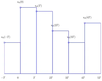
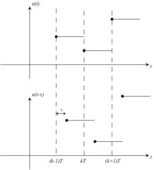
Most of the system (plants) we will be trying to control in the world are inherently continuous-time, and we would like to use discrete-time control. The biggest issue is how we are going to be able to model the continuous-time plant as a discrete-time plant. The most common method is to assume we have discrete-time signals, ud(kT), which we model as impulse signals which that

only exist at the sample times kT. Speciﬁcally, we can writeud(kT) as

ud(kT) = . . .+ud(−T)δ(t+T) +ud(0)δ(t) +ud(T)δ(t−T) +ud(2T)δ(t−2T) +. . .

where the delta functions are continuous-time delta functions. This is shown graphically in Figure 2.

−T

ud(−T)

0

ud(0)

T

ud(T)

2T

ud(2T)

3T

ud(3T)

4T

ud(4T)

5T

Figure 2: Impulse model of a discrete-time signal.

From these impulse signals we need to generate a continuous-time signal as an input to the plant, Gp(s). The most common way to do this is by the use of a zero order hold(zoh), which

constructs a continuous-time signal by holding the value of u(kT) constant for time intervals kT ≤ t < (k+ 1)T. The impulse response of the zero order hold is gzoh(t) = u(t)−u(t−T).

Let’s call the continuous-time output of the zero order hold uc(t), so we have

uc(t) = gzoh(t)∗ud(kT)

= gzoh(t)∗[. . .+ud(−T)δ(t+T) +ud(0)δ(t) +ud(T)δ(t−T) +ud(2T)δ(t−2T) +. . .]

(29)

−T ud(−T)

0

ud(0)

T ud(T)

2T

ud(2T)

3T

ud(3T)

4T

ud(4T)

[image:29.612.131.481.86.363.2]

5T

Figure 3: Continuous-time signal uc(t) as input to the plant. The value of the signal is held

constant over the sample interval T.

How let’s look at some of these convolutions,

gzoh(t)∗[ud(−T)δ(t+T)] = ud(−T)gzoh(t)∗δ(t+T) = ud(−T)gzoh(t+T) =ud(−T)[u(t+T)−u(t)]

gzoh(t)∗[ud(0)δ(t)] = ud(0)gzoh(t)∗δ(t) =ud(0)gzoh(t) =ud(0)[u(t)−u(t−T)]

gzoh(t)∗[ud(T)δ(t−T)] = ud(T)gzoh(t)∗δ(t−T) =ud(0)gzoh(t−T) =ud(T)[u(t−T)−u(t−2T)]

Hence we have the input to the continuous-time plant

uc(t) =. . .+ud(−T)[u(t+T)−u(t)] +ud(0)[u(t)−u(t−T)] +ud(T)[u(t−T)−u(t−2T)] +. . .

This is a staircase function, where we have ”ﬁlled in” the times between samples with the value of the sample at the beginning of the interval. This is shown graphically in Figure 3. It should be pointed out that a zero order hold is not the only method that can be used to convert a discrete-time signal to a continuous-time signal, but it is the most commonly used method, and is the method we will use when we convert continuous-time state equations to discrete-time state equations.

(30)

What we want is the discrete-time transfer function that corresponds to the productGzoh(s)Gp(s),

or

Gp(z) =Z {Gzoh(s)Gp(s)}

Using properties of the Laplace transform we have

Gzoh(s) =L {gzoh(t)}=L {u(t)−u(t−T)}=

1 s −

e−sT

s So we have

Gp(z) =Z

1 s −

e−sT

s

Gp(s)

We can use this formula directly, but it there is a common trick we can use to make things a bit easier. Let’s write

Gzoh(s)Gp(s) =

1 s −

e−sT

s

Gp(s) =

1−e−sTGi(s)

where we have deﬁned

Gi(s) =

Gp(s)

s

Now we know from Laplace transforms that e−sT corresponds to a time delay of T, hence we have

L−1_e−sT_G

i(s) =gi(t−T)

and then taking z-transforms

Z {gi(t−T)}=Z {gi(kT −T)}=z−1Gi(z)

Where

Gi(z) =Z {gi(kT)}

Finally, we will use the Linearity property of the z-transform, Gp(z) =Z

Gi(s)−e−sTGi(s) =Gi(z)−z−1Gi(z) =

1−z−1Gi(z)

R(z)

G_p(z) G_c(z)

G

_zoh

(s)

G_p(s) Y(z)

H(z)

+ +

-Σ

}

G

_p

(z)

(31)

which is the answer we want. In summary, the discrete-time transfer function that models the zero order hold and the continuous- time plant is given by

Gp(z) =

1−z−1Z

Gp(s)

s

Example.Consider the continuous-time plant with transfer function Gp(s) = _s₊₁1 . What is the

equivalent discrete-time transfer function for the plant in series with a zero order hold? We have Gp(z) =

1−z−1Z

1 s(s+ 1)

so

Gi(s) =

1 s(s+ 1) =

1 s −

1 s+ 1 and

gi(t) =u(t)−e−tu(t)

The sampled version is given as

gi(kT) = u(kT)−e−kTu(kT)

with z-transform

Gi(z) =

z z−1−

z z−e−T =

z(1−e−T₎

(z−1)(z−e−T₎

Finally, we have

Gp(z) =

z−1

z Gi(z) =

1−e−T

z−e−T

Example. Consider the continuous-time plant with transfer function Gp(s) = 1_s. What is the

equivalent discrete-time transfer function for the plant in series with a zero order hold?We have Gp(z) =

1−z−1Z !

1 ss

"

so

Gi(s) =

1 s2 and

gi(t) =tu(t)

The sampled version is given as

gi(kT) = kT u(kT)

with z-transform

Gi(z) =

T z (z−1)2 Finally, we have

Gp(z) =

z−1

(32)

1.12

Final Notes

We have focused on using transfer functions in terms of z, such as H(z) = K(z−a)(z−b)

(z−c)(z−d) =

K(z2 −(a+b)z+ab) z2 −(c+d)z+cd

This form is useful for determining poles and zeros and determining the time-response of the sys-tem. However, when implementing controllers (ﬁlters) in discrete-time, it is far more convenient to write things in terms ofz−1, which represents a delay of one time sample. For implementation purposes, we would write this transfer function as

H(z) = K(1−(a+b)z

−1₊_abz−2₎

1−(c+d)z−1+cdz−2 =

K(1−az−1)(1−bz−1) (1−cz−1)(1−dz−1)

(33)

2

Transfer Function Based Discrete-Time Control

Just as with continuous-time control, we can choose to utilize a transfer function approach or a state variable approach to control. In this chapter we will utilize the transfer function ap-proach, while in the remainder of these notes we will utilize the state variable approach. In this brief chapter we ﬁrst discuss implementing discrete-time transfer functions, then talk about some common conventions used in control systems, and then discuss common control algorithms.

2.1

Implementing Discrete-Time Transfer Functions

Just as in continuous-time we will represent signals in either the time domain or the transform domain, which in this case is the z-transform domain. A simple input-output transfer function block is shown in Figure 5. While in the continuous time-domain it might be somewhat diﬃcult to solve for the output in terms of the input in the time-domain, in the discrete-time domain we can just use the recursive relationship from the transfer function. Speciﬁcally, if we have the transfer function G(z), then we can write it as

G(z) = Y(z) U(z) =

b₀+b₁z−1 +b₂z−2 +· · ·+bmz−m

1 +a₁z−1+a₂z−2+· · ·+anz−n

where n ≥m. Converting this to the time domain, the output y(k) can be written in terms of previous output values and the current and previous input values as

y(k) = −a₁y(k−1)−a₂y(k−2) +· · · −any(k−n) +b0u(k) +b1u(k−1) +...+bmu(k−m)

This is an Infinite Impulse Response (IIR) filter, since the output at any time depends on both previous outputs and previous inputs. If the output depended only on previous inputs it would be a Finite Impulse Response (FIR) filter.

G(z)

Y(z)

U(z)

Figure 5: Discrete-time transfer function, G(z) = Y_U(₍z_z)₎. Discrete-time transfer functions are often implemented in terms of the diﬀerence equation they represent.

2.2

Not Quite Right

At this point we need to stop and think a little bit about what we are doing, and the common conventions used in control systems. Let’s assume we have a simpliﬁed version of the above expression, which we will write using the explicit dependence on the sample interval T,

(34)

Now we have to examine w