Results of pig carcass classification according to SEUROP in the Czech Republic

Pigs and dairy cows are the two main industries of livestock production in the Czech Republic (CR) and in the European Community (EC) as a whole. Of the total annual per capita meat consumption in the CR (81 kg), in the EC (92 kg) and worldwide (42 kg) pig meat accounts for 54% (43.5 kg), 47% (42.7 kg) and 39% (16.4 kg), respectively. Long-term forecasts indicate that the production and consumption of pig meat in the EC will slowly grow by about 3% to 4% by 2013. In accordance with the common agricultural policy reform, which is in the process of realization, increased attention will be paid to food production. Consequently, issues associated with the identification, classification and quality of pig carcasses will be of increased importance.

According to Kirton (1989) pig classification is the most objective of the various systems applied to pig, sheep and cattle carcasses, because it is the animal to which it is easiest to apply objective clas-sification methods. One reason for this is that it has more uniform fat cover than other species.

The conventional method of pig carcass classifi-cation (FOM, SKG II) was analysed by Matzke et al. (1986), the AutoFOM system based on ultrasonic measurements was described by Brøndum et al. (1998), Busk et al. (1999), and the accuracy of FOM instruments used in on-line pig carcass classifica-tion in the CR was detailed by Šprysl et al. (2007) and others.

The accuracy of the EU reference dissection method for pig carcass classification in four

dif-Supported by the Ministry of Agriculture of the Czech Republic (Project No. MZE 0002701403).

Results of pig carcass classification according to

SEUROP in the Czech Republic

J. Kvapilík

_{, J. Přibyl}

_{, Z. Růžička}

_{, D. Řehák}

1_{Institute of Animal Science, Prague-Uhříněves, Czech Republic} 2_{Czech-Moravian Breeders’ Corporation, Prague, Czech Republic}

ABSTRACT:Through data analysis of 7 571 883 pig carcasses slaughtered from 2004 to 2007 the means of quality classes (QC) 2.32, lean meat percentage (LM) 55.83%, carcass weight (CW) 87.21 kg, muscle thickness (MT) 61.95 mm and fat thickness (FT) 15.95 mm were determined. The highest correlation coefficients are between QC and LM (r = –0.920), LM and FT (–0.900) as well as QC and FT (0.828), the lowest between FT and MT (r = –0.084). Quality class as the dominant indicator is influenced mainly by LM, which explains from 77% to 89% of variability in the case of linear regression. Among the eight methods of pig carcass clas-sification the FOM apparatus was used the most frequently (46.5% carcasses) followed by the ULTRA-FOM 300 apparatus (15.6%), another apparatus (13.2%) and by the IS-D-05 unit (9.8%). In the statistical models used all effects (differences) are statistically significant because of the large size of the data set. The results from the separate evaluation of each cross-classified effect are that EV has the largest influence and year-season and methods have a smaller influence. The time trend (42 months) documents stable CW and MT, a slight increase in LM and improvement of QC. The estimated results indicate the successful introduction of pig carcass classification in the CR after accession to the EU.

ferent European countries was estimated by Nissen et al. (2006). Characteristics of selected carcasses were hot carcass weight, fat and muscle thickness and lean meat content. The accuracy expressed by the repeatability (0.87), reproducibility standard deviation (1.10) and reliability (0.87) was high.

Methods of evaluation of carcasses are under permanent development. Bahelka et al. (2007) ana-lysed the influence of sex and slaughter weight on carcass quality. Vítek et al. (2008) documented the improvement of carcass classification by add-ing additional characteristics. Kusec et al. (2008) pointed out the optimal slaughter weight with growth curve. Lean and fat development was an-alysed with magnetic resonance tomography by Margeta et al. (2007).

According to Olsen et al. (2007) the quality of the calibration, maintenance of instruments, training of operators, working conditions and other factors in-fluencing routine work are important for the results of pig carcass classification (fat and muscle thick-ness and lean meat content). Variations between operators were more important than the variation between copies of the same type of instrument. These results were found in thirteen EC-countries including the CR.

Pulkrábek et al. (2003) analyzed the relation-ships among individual characteristics included in the process of pig carcass evaluation based on lean meat content in the CR. The average slaughter weight and lean percentage were 112.8 ± 0.082 kg and 54.86% ± 0.022%, respectively. The improve-ment of the lean meat content in the last 10 years could be expressed as equal to 1.5 classes of the 6-point classification scale. It was satisfying that most carcasses (97.3%) were included in the weight range required for the classification system, i.e. from 60–120 kg. Good quality of carcass was con-firmed by classification results when 86.3% of car-casses were placed in classes S, E, and U.

In the calculation of genetic parameters of pig carcass composition and quality e.g. Van Wijk et al. (2005) found the average weight of 1 791 pig carcasses to be 86.2 kg and the average lean meat content of 1 645 carcasses to amount to 50.7% and muscle thickness to 59.3 mm.

High lean meat content is characteristic of Belgian pig breeds. According to Castryck (2007) the aver-age lean meat content reached 59.93%. Out of all the pig carcasses 51.69% were included in class S, 42.73% in class E, 5.62% in class U, 0.31% in class R and 0.01% in class O.

Slovenian results for pig carcass classification ac-cording to SEUROP for the years from 1996 to 2004 were presented by Čandek-Potokar et al. (2004). In these years, a significant increase in average lean meat percentage was noted (51.9% in 1996 vs. 55.9% in 2004). As a consequence the percentage of pig carcasses being graded into S and E classes was almost tripled from 1996 to 2004 (21.3% to 58.2%, respectively).

From 1997 to 2007 the quality of pig carcasses classified in Austria improved (class S +3.07% to 46.37%, class E +4.86% to 45.47%). There was also an increase of 19.9% in the number of slaughtered pigs (AMA Austria, 2008).

Lean meat content is one of the goals of pig breed-ing. In the Czech Republic this goal is set between 52% for the very good reproductive pig line and 64% for the Pietrain breed (Pražák, 2001). Equivalent data for the lean meat content are also reported in other countries.

The objective of this article is an analysis of the CR national database, of the main traits investigated within pig carcass classification, and an assessment of the accuracy of the methods of classification.

MATERiAl And METhOdS

From May 2004 to October 2007 the central animal register of the Czech-Moravian Breeder’s Corporation recorded a total of 7 730 397 slaugh-tered pigs. The statistical evaluation includes only pig carcasses with complete data in the respective quality class and meeting the following interval of traits:

– quality classes (QC) S, E, U, R, O and P (1 to 6); – carcass weight (CW) 40 to 150 kg;

– lean meat percentage (LM) 30 % to 70 %; – fat thickness (FT) 5 to 60 mm;

– muscle thickness (MT) 20 to 120 mm.

After purging incomplete and less reliable data, the number of pig carcasses was reduced to 7 668 924 pieces, or 99.2% of the original size of the set. Only 0.8% of carcasses were eliminated from analysis because of incomplete or unreliable data. The pig carcasses were classified by 311 evaluators (EV) (on average 24 258 carcasses per EV).

weight under 60 kg belong to the class N, and above 120 kg they belong to the class T.

Pig carcass classification is derived from the per-centage of lean meat content, which is determined on the basis of muscle and/or fat share measure-ment according to regression equations. The Czech Regulation (No. 194/2004) establishes eight classi-fication methods for the evaluation of pig carcasses according to the following numbered key:

– apparative method: units FOM (1), HGP (2), UFOM-300 (3), IS-D-05 (7) and IS-D-15 (8) – two-point method – electromechanical measu-

re (4)

– other apparatus (5)

– two-point method – table (6)

According to regulations for quality classes N and T only CW was estimated. For classes S to P CW and LM, both MT and FT, were detected. Data process-ing classes S to P were marked by numbers 1 to 6 (from the best to the worst classification).

Statistical traits were analysed by GLM in SAS according to several statistical models with com-binations of cross-classified and regression effects according to the overall model equation:

y = CCE + REG + e

where:

y = sequential trait evaluation (QC, LM, MT, FT, CW)

CCE = sequentially used cross-classified effects of EV, year × season (YS) and classification method REG = alternatively used linear and quadratic regression

on LM, MT, FT, CW and YS e = random residual effect

RESUlTS And diSCUSSiOn

Average characteristics and correlation relations

Classification of QC is a step by step procedure. EVs in slaughterhouses with the help of estab-lished methods determine the MT and FT. From the prediction equations values are calculated for LM. Values of LM together with CW are predic-tors of QC.

The majority of the pig carcasses met the condi-tions for submission into the basic quality classes

Table 1. Numbers and weight of pig carcasses in the quality classes

Quality class Number of carcasses Carcass weight (kg)

count (%) AVG SD

S to P 7 571 883 98.7 87.2 10.7

N 67 941 0.9 53.5 5.1

T 29 100 0.4 126.6 6.5

Total 7 668 924 100.0 87.1 11.4

SD =standard deviation

Table 2. Main statistical characteristics of pig carcasses (n = 7 571 883)

Trait AVG SD CV (%) SE

QC (1 to 6) 2.32 0.745 32.1 0.0003

LM (%) 55.83 3.48 6.2 0.0013

CW (kg) 87.21 10.66 12.2 0.0039

MT (mm) 61.95 9.02 14.6 0.0033

FT (mm) 15.95 4.66 29.2 0.0017

of the scale of the “SEUROP” system. In class “N” with a carcass weight of less than 60 kg. 67 941 carcasses (0.9%) were registered with an average weight 53.5 kg and in class “T” (over 120 kg) 29 100 carcasses (0.4%) were registered with 126.6 kg (Table1). This means that the share of pigs with extremely low or high carcass weight represents only 1.3% of all the pigs slaughtered. The aver-age pig carcass weight in the CR (87.2 kg) was for example higher than in Slovenia (81 to 83 kg; Čandek-Potokar et al., 2004) and comparable with the Netherlands (86.2 kg, Van Wijk et al., 2005).

Because the majority of the pig carcass charac-teristics (LM, FT, MT) in the classes “N” and “T” are not recorded, the data of 7 571 883 and 98.7% classified carcasses in classes “S” to “P” (Table 2) are evaluated and discussed in the following section. The variability of the determined aver-ages was highest by QC of carcasses (coefficient of variation 32.1%) and FT (29.2%), the lowest by LM (6.2%).

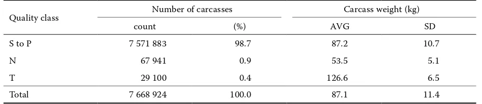
Some of the relations among the pig carcass in-dicators are illustrated in Figure 1. The highest correlations (Table 3) are between QC and LM

(r = –0.920), LM and FT (–0.900) as well as QC and FT (0.828), the lowest between FT and MT (r = –0.084). Because of the high sample size all the relations are statistically highly significant.

Quality classes (lean meat percentage) and carcass weight

For submission to the QC the pig carcass hot weight (from 60 to 120 kg) and the LM content are determining factors. For the class “S” LM share requires 60% and more, for class “P” less than 40% (Table 4). For the classes “E” to “O” between 60% and 40% are set the five-percentage intervals of lean meat share. The LM average of all quality classes is 55.8% and ranges between 61.1% in class “S” and 37.4% in class “P”.

More than one half of the pig carcasses (54.0%) satisfied the conditions for class “E” and almost one third (30.3%) of carcasses for class “U”. In the best quality class “S” 10.1% could be included. Whereas in “O” and “P”, the two worst classes, there are only 0.5% and 0.1% of the classified pig 0

10 20 30 40 50 60 70 80 90 100 110

32 34 36 38 40 42 44 46 48 50 52 54 56 58 60 62 64 66 68 70 LM (%)

(kg,

mm)

Figure 1. CW, MT, FT according to LM of pig carcasses

Table 3. Pearson correlation coefficients (n = 7 571 883)

Trait FT (mm) MT (mm) CW (kg) LM (%)

QC (1 to 6) 0.828* –0.301* 0.257* –0.920*

LM (%) –0.900* 0.320* –0.275*

CW (kg) 0.388* 0.298*

MT (mm) –0.084*

carcasses. Average QC (S to P = 1 to 6) represents 2.32 (Table2), which is a slightly worse classifica-tion than the average of class “E” (Table 4). The pig carcass share in the quality classes S, E und U reached 94.4%, which is by 8.1% more than is shown by Pulkrábek et al. (2003) for the Czech pig population, but by 5.3% less than in 2006 in Belgian pigs (Castryck, 2007). All differences among pig

carcass trait averages in individual quality classes (LM, CW, FT and MT) are significant.

The average LM of pig carcasses in the CR (55.8%) is among the values specified for pig breeding goals (52 to 64%) and is lower for example than in Belgium in 2006 (59.93%; Castryck, 2007) and comparable with Slovenia in 2004 (55.9%; Čandek-Potokar et al., 2004).

Table 4. Traits of pig carcasses in quality classes “S” to “P”

Trait Quality class of pig carcasses

2

S (1) E (2) U (3) R (4) O (5) P (6) total3

Pig carcasses (%) 10.1 54.0 30.3 5.0 0.5 0.1 100.0

LM (%) AVG 61.1 57.3 53.0 48.2 43.2 37.4 55.8

SD1 _{1.0 1.4 1.4 1.3 1.3 2.2 3.5}

CW (kg) AVG 82.8 85.9 89.9 93.5 95.7 97.0 87.2

SD1 _{10.2 10.2 10.4 10.7 11.4 12.4 10.7}

FT (mm) AVG 9.9 14.1 19.4 25.5 32.1 39.5 16.0

SD1 _{1.7 2.4 3.0 3.6 3.4 4.2 4.7}

MT (mm) AVG 67.8 62.8 59.7 56.2 51.7 50.4 62.0

SD1 _{8.6 8.3 8.8 10.0 9.9 8.0 9.0}

1_{standard deviation;} 2_{all differences between quality classes are significant (P < 0.001);} 3_{100% = 7 571 883 pig carcasses}

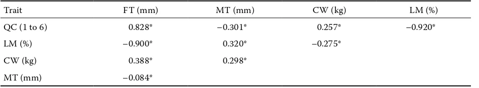
Table 5. The main traits of pig carcasses according to carcass weight

Indicator Pig carcass weight (kg)

2

< 70 70–79.9 80–89.9 90–99.9 100–109.9 ≥ 110 total3

Carcasses (%) 5.1 19.9 36.0 27.1 9.8 2.1 100.0

QC AVG 2.0 2.1 2.3 2.4 2.6 2.8 2.32

SD1 _{0.65 0.68 0.71 0.75 0.79 0.85 0.745}

CW (kg) AVG 66.2 75.8 85.0 94.3 103.8 113.7 87.2

SD1 _{2.7 2.8 2.8 2.8 2.7 2.9 10.7}

LM (%) AVG 57.6 56.8 56.1 55.2 54.3 53.2 55.8

SD1 _{3.0 3.1 3.3 3.5 3.7 4.1 3.5}

MT (mm) AVG 55.6 59.0 61.6 63.9 65.8 67.4 62.0

SD1 _{8.6 8.3 8.4 8.8 9.4 10.2 9.0}

FT (mm) AVG 12.5 14.0 15.6 17.1 18.8 20.6 16.0

SD1 _{3.7 3.9 4.2 4.5 4.9 5.4 4.7}

The largest share of pig carcasses, with an average weight of 87.2 kg, belongs in the weight interval be-tween 80 and 90 kg (36.0%) followed by the intervals 90 to 100 kg (27.1%) and 70 to 80 kg (19.9%). With carcass weight increase there has been an explicit trend to thicker muscle and fat and to a slow de-crease in the percentage of lean meat (Table 5).

Pulkrábek at al. (2006) found a comparable lean meat proportion (55.38%) (in the Czech pig popu-lation), but about 3.6 kg and 4.0% lower average carcass weight.

Classifier, methods and results of pig carcass classification

On average there were 24 258 classified pig carcasses per one EV with fluctuations between 1 and 312 353 animals. From a total of 311 EV 36 (11.6%) of them classified less than 100 animals, 94 (30.2%) less than 1 000 animals and 187 (60.1%) less than 10 000 animals. In the majority of cases the EV used only one method and identification of each EV is also the identification of the batch and slaughter place. Only in 50 cases did one EV use more than one method (in 18.3% it was possible to compare two methods from one EV).

Out of the eight methods of pig carcass classifi-cation (Table 6) the most frequently used (46.5% of pig carcasses) was Method 1 (FOM apparatus)

followed by Method 3 (ULTRA-FOM 300 appara-tus, 15.6%), 5 (other apparaappara-tus, 13.2%), 7 (IS-D-05 unit, 9.8%) and 4 (two-point method, 6.4%). With the help of the remaining two methods only 2.2% (Method 2, HGP apparatus) and 0.2% (Method 8, IS-D-15 unit) of pig carcasses were classified.

Because of the large data set, even the least fre-quently used method has enough data for evaluation; all effects are statistically significant by all methods.

Large differences in estimated averages, and espe-cially in the variability of evaluated traits (Table6), are seen among the particular methods. In all traits Method 8 has the smallest SD, which differs vis-ibly from the other methods. Method 4, 6 and 8 show much higher averages for MT than the other methods. But LM averages, calculated by prediction equations specific to each method, are more similar for all methods. From this point of view, Method 4, 6 and 8 systematically differ from the other methods in the prediction of average MT. Method 8 underval-ued differences among animals in all observed traits. According to Figure 2 the mean MT shows the great-est variation among the classification methods.

Measurement of muscle thickness and fat thickness

Classification methods are differently sensitive to the systematic effects of the EVs and year and

sea-Table 6. The main traits of pig carcasses according to the method of classification

Trait Method of classification

1 2 3 4 5 6 7 8

Carcasses (%)1 _{46.5 2.2 15.6 6.4 13.2 6.1 9.8 0.2}

QC (1 to 6) AVG 2.27 2.33 2.42 2.40 2.39 2.34 2.27 2.33

SD2 _{0.68 0.76 0.86 0.76 0.75 0.81 0.76 0.43}

LM (%) AVG 56.1 55.8 55.3 55.5 55.5 55.5 56.1 54.8

SD2 _{3.1 3.6 4.1 3.5 3.5 3.9 3.5 0.5}

MT (mm) AVG 61.6 58.7 56.2 70.2 60.5 69.3 65.0 71.6

SD2 _{7.6 8.0 8.0 8.5 9.8 7.1 9.3 3.6}

FT (mm) AVG 16.0 15.9 17.1 16.8 14.0 16.4 15.7 16.6

SD2 _{4.0 4.4 5.7 5.1 4.4 5.7 4.2 1.7}

CW (kg) AVG 87.5 86.6 86.5 86.9 86.7 88.9 87.2 83.7

SD2 _{10.7 10.9 10.5 10.8 10.5 11.1 10.7 7.5}

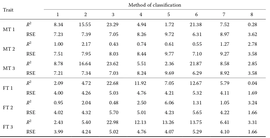
son (Table 7). The EVs explain the variability in MT in the different methods from 1.72% (Method 5) to 23.29% (Method 3). The YS explains for MT in the different methods from 0.55% (Method 6) to 2.17% (Method 2) of variability. Both effects together ex-plain for MT from 2.36% to 23.62% of variability. To these values correspond reciprocally the residual

standard deviations in each method (RSE). Method 8 is not considered in the comparison, because only two EVs used it. FT was influenced less, but also here in Method 3 EVs play a much greater role than in the other methods.

From this point of view the least influence of EVs on results was in Method 5 for MT and in 50

60 70 80 90

1 2 3 4 5 6 7 8

Classification method

LM

(%),

MT

(mm)

and

CW

(kg)

1.0 1.5 2.0 2.5 3.0

Quality

class

LM (%) MT (mm) CW (kg) QC Figure 2. Classification method and indices of pig carcasses

Table 7. Accuracy of MT and FT measurement by different methods

Trait Method of classification

1 2 3 4 5 6 7 8

MT 1 R

2 _{8.34 15.55 23.29 4.94 1.72 21.38 7.52 0.28}

RSE 7.23 7.39 7.05 8.26 9.72 6.31 8.97 3.62

MT 2 R

2 _{1.00 2.17 0.43 0.74 0.61 0.55 1.27 2.78}

RSE 7.51 7.95 8.03 8.44 9.77 7.10 9.27 3.58

MT 3 R

2 _{8.78 16.64 23.62 5.51 2.36 21.87 8.58 2.85}

RSE 7.21 7.34 7.03 8.24 9.69 6.29 8.92 3.58

FT 1 R

2 _{2.09 4.72 22.68 11.92 7.05 12.67 5.79 0.04}

RSE 4.00 4.26 5.03 4.76 4.21 5.32 4.11 1.69

FT 2 R

2 _{0.95 2.04 0.48 2.50 6.06 1.31 1.05 3.24}

RSE 4.02 4.32 5.70 5.01 4.23 5.65 4.22 1.66

FT 3 R

2 _{2.43 5.40 22.98 12.13 13.26 13.75 6.41 3.31}

RSE 3.99 4.24 5.02 4.76 4.07 5.29 4.10 1.66

1 = model includes only the effect of EV; y = EV + e 2 = model includes only the effect of YS; y = YS + e 3 = model includes both effects of EV + YS; y = EV + YS + e R2 _{= determination coefficient of the model}

Method 1 for FT. Method 5 was used by 17 EVs only with a high quantity of evaluated animals for each. Therefore results can also be influenced by the personal experiences of EVs.

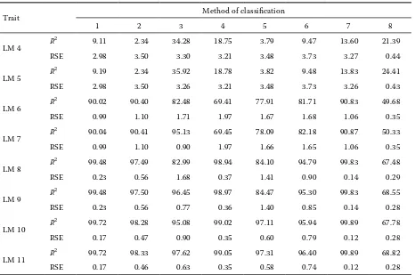
Prediction of lean meat percentage

The main results of the prediction of lean meat percentages are summarised in Table 8. Using only one linear regression coefficient, FT (Model 6) pre-dicts LM much better (determination coefficients from 49.68% to 90.83%) than MT (Model 4) (de-termination coefficients from 2.34% to 34.28%). The dependence of LM on FT should not neces-sarily be linear, mainly in extremes of the range of

variations; therefore the quadratic regression was also included. Including the quadratic regression (Model 7), except for Method 3, it does not have a sizable impact on evaluation. The prediction ac-cording to FT is best for Method 3 and worst for Method 8; accordingly MT is best for Method 3 and worst for Method 2. The prediction using both linear regression coefficients together (Model 7) is more similar for all methods except Method 8. The determination coefficients ranged from 82.99% to 99.83%. When using the quadratic regression, the determination coefficients ranged from 84.47% to 99.83%. The highest precision of prediction was observed for Methods 7, 1, 4 and 2.

Additionally including the systematic effects of EV and YS (Model 10) in a prediction also improves Table 8. Accuracy of LM prediction by different methods

Trait Method of classification

1 2 3 4 5 6 7 8

LM 4 R

2 _{9.11 2.34 34.28 18.75 3.79 9.47 13.60 21.39}

RSE 2.98 3.50 3.30 3.21 3.48 3.73 3.27 0.44

LM 5 R

2 _{9.19 2.34 35.92 18.78 3.82 9.48 13.83 24.41}

RSE 2.98 3.50 3.26 3.21 3.48 3.73 3.26 0.43

LM 6 R

2 _{90.02 90.40 82.48 69.41 77.91 81.71 90.83 49.68}

RSE 0.99 1.10 1.71 1.97 1.67 1.68 1.06 0.35

LM 7 R

2 _{90.04 90.41 95.13 69.45 78.09 82.18 90.87 50.33}

RSE 0.99 1.10 0.90 1.97 1.66 1.65 1.06 0.35

LM 8 R

2 _{99.48 97.49 82.99 98.94 84.10 94.79 99.83 67.48}

RSE 0.23 0.56 1.68 0.37 1.41 0.90 0.14 0.29

LM 9 R

2 _{99.48 97.50 96.45 98.97 84.47 95.30 99.83 68.55}

RSE 0.23 0.56 0.77 0.36 1.40 0.85 0.14 0.28

LM 10 R

2 _{99.72 98.28 95.08 99.02 97.11 95.94 99.89 67.78}

RSE 0.17 0.47 0.90 0.35 0.60 0.79 0.12 0.28

LM 11 R

2 _{99.72 98.33 97.62 99.05 97.31 96.40 99.89 68.82}

RSE 0.17 0.46 0.63 0.35 0.58 0.74 0.12 0.28

4 = model includes linear regression on MT; y = MT + e

5 = model includes quadratic regression on MT; y = MT + MT2 _{+ e} 6 = model includes linear regression on FT; y = FT + e

7 = model includes quadratic regression on FT; y = FT + FT2 _{+ e} 8 = model includes linear regression on MT and FT; y = MT + FT + e

9 = model includes quadratic regression on MT and FT; y = MT + MT2 _{+ FT + FT}2 _+ e

10 = model includes linear regression on MT and FT and EV + YS effect; y = MT + FT + EV + YS + e

the prediction. Large improvement is seen espe-cially for Methods 3 and 5. This implies that the individuality of EV influenced the prediction of LM in these methods.

Prediction of quality class

Quality class is influenced mainly by LM, which explains from 77.14% to 88.71% of variability in the case of linear regression (Table 9). Including the quadratic regression (Model 13) plays a role only in Method 8, which improves the determination coefficient from 77.14% to 90.45%. CW influenced QC to a much lesser extent. In Method 8 it explains 20.92% of variability in the case of linear regression and 25.92% of variability in quadratic regression.

In the other methods it explains CW from 1.81% to 10.57% of variability. Including quadratic regres-sion does not improve the results.

Including regression on both LM and CW does not differ practically from using regression on LM only (comparison of Models 12 with 16 and 13 with 17). The inclusion of cross-classified effect of EV and YS does not influence the results either (Models 18 and 19).

differences between methods of classification

Table 6 shows rough averages for measured val-ues. In Table 10 are summarised averages for meth-ods corrected from all effects influencing the traits. Table 9. Accuracy of QC prediction by different methods

Trait Method of classification

1 2 3 4 5 6 7 8

QC 12 R

2 _{81.80 85.51 88.71 85.51 84.77 84.89 85.40 77.14}

RSE 0.29 0.29 0.29 0.29 0.29 0.31 0.29 0.20

QC 13 R

2 _{81.80 85.51 88.75 85.54 84.79 85.17 85.40 90.45}

RSE 0.29 0.29 0.29 0.29 0.29 0.31 0.29 0.13

QC 14 R

2 _{7.14 8.42 10.57 1.81 7.71 3.31 5.84 20.92}

RSE 0.65 0.73 0.82 0.76 0.72 0.79 0.74 0.38

QC 15 R

2 _{7.22 8.42 10.57 1.90 7.80 3.34 5.90 25.92}

RSE 0.65 0.73 0.82 0.76 0.72 0.79 0.74 0.37

QC 16 R

2 _{81.80 85.51 88.72 85.51 84.77 84.92 85.40 77.15}

RSE 0.29 0.29 0.29 0.29 0.29 0.31 0.29 0.20

QC 17 R

2 _{81.80 85.51 88.76 85.54 84.80 85.19 85.40 90.51}

RSE 0.29 0.29 0.29 0.29 0.29 0.31 0.29 0.13

QC 18 R

2 _{81.85 85.53 88.74 85.57 84.87 85.62 85.40 77.18}

RSE 0.29 0.29 0.29 0.29 0.29 0.31 0.29 0.20

QC 19 R

2 _{81.85 85.53 88.78 85.59 84.90 85.81 85.41 90.54}

RSE 0.29 0.29 0.29 0.29 0.29 0.30 0.29 0.13

12 = model includes linear regression on LM; y = LM + e

13 = model includes quadratic regression on LM; y = LM + LM2 _{+ e} 14 = model includes linear regression on CW; y = CW + e

15 = model includes quadratic regression on CW; y = CW + CW2 _{+ e} 16 = model includes linear regression on LM and CW; y = LM + CW + e

17 = model includes quadratic regression on LM and CW; y = LM + LM2 _{+ CW + CW}2 _{+ e}

18 = model includes linear regression on MT and FT and EV + YS effect; y = LM + CW + EV + YS + e

Due to the large quantity of the data all means have very small standard errors. Table 11 documents the values of determination coefficients of models and residual standard deviations.

The trends of the LS means (Table 10) are similar to the rough data in Table 6. Method 8 has very large differences for MT from the other methods. Averages for QC and LM are practically the same for all methods. MT is largest (except Method 8) for Method 4 and 6 and smallest for Method 5, 1 and

3. For FT and CW there are smaller differences between the methods.

When judging each cross-classified effect sep-arately, EV has the largest influence and YS and methods have the smallest influence. For MT it is found that the method (Model 23) and especially EV (Model 1) are much more important than YS (Model 2). Explained variances in complex Models 20, 21 and 22 are similar to the models within each methods presented in previous tables.

Table 10. LSM averages of methods corrected by all effects

Trait Method of classification

1 2 3 4 5 6 7 8

QC 20 AVG 2.320 2.330 2.320 2.320 2.310 2.300 2.310 2.050

SE 0.002 0.003 0.003 0.002 0.002 0.002 0.002 0.004

LM 21 AVG 55.840 56.100 55.850 55.160 54.860 55.050 56.060 54.720

SE 0.005 0.008 0.006 0.005 0.005 0.005 0.005 0.008

MT 22 AVG 61.070 62.390 61.400 69.350 60.000 67.910 64.190 71.720

SE 0.055 0.089 0.076 0.057 0.059 0.058 0.059 0.098

FT 22 AVG 15.910 16.760 16.750 15.470 13.760 16.660 16.280 15.800

SE 0.031 0.050 0.042 0.032 0.033 0.032 0.033 0.055

CW 22 AVG 87.600 87.920 90.100 87.580 87.850 87.220 86.400 85.850

SE 0.074 0.120 0.102 0.077 0.079 0.078 0.080 0.132

20 = model includes quadratic regression on LM and CW and EV + YS + Method effect; y = LM + LM2 _{+ CW + CW}2 _{+ EV +} YS + Method + e

21 = model includes quadratic regression on MT and FT and EV + YS + Method effect; y = MT + MT2 _{+ FT + FT}2 _{+ EV +} YS + Method + e

22 = model includes the effects of EV + YS + Method; y = EV + YS + Method + e

Table 11. Variability and residual standard deviation for data with all methods

Model QC LM MT FT CW

1 R

2 _{4.30 5.14 23.21 11.89 3.00}

RSE 0.73 3.39 7.90 4.38 10.51

2 R

2 _{0.69 0.85 0.45 1.37 0.68}

RSE 0.74 3.47 9.00 4.63 10.63

23 R

2 _{0.78 0.92 17.75 3.50 0.33}

RSE 0.74 3.47 8.18 4.58 10.65

20, 21, 22 R

2 _{84.74 96.46 25.62 13.21 3.60}

RSE 0.29 0.66 7.78 4.35 10.47

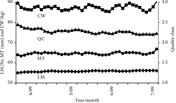
development of pig carcasses traits in time

Although the time period of the classification of pig carcasses is relatively short, Table 12 shows regression coefficient dependences of evaluated traits on time, expressed in year × month (YM) classes. All regres-sion coefficients are statistically significant, but the values are very small. The time trend (42 months) in Figure 3 shows stable CW and MT, a slight increase in LM and improvement of QC. In the graphic expres-sion of the time trend, YM in Model 24 was used as a cross-classified effect with 43 YM levels.

COnClUSiOnS

The objective of the present study was to analyse the main results and to describe the accuracy of pig carcass classification methods. The average of the values deter-mined within the classification of more than 7 million pig carcasses (QC, CW, LM, MT and FT) is compara-ble with the same values found in the other EC states. 94.4% of all pig carcasses were included in the three best-quality classes (S, E and U), which shows quite good quality of pigs in the CR. Because of the large data set the differences in the average results among the 8

methods and 311 classifiers are statistically significant. Classification methods differ in variability and partly in averages of evaluated traits, nevertheless the accuracy of methods (with the exception of Method 8) as well as classifiers, when all simultaneously acting effects are included in evaluation, is comparable.

Acknowledgement

The authors thank Mr. Patrick Noel O’Brien for the language revision of this manuscript.

REFEREnCES

Bahelka I., Hanusová E., Peškovičová D., Demo P. (2007): The effect of sex and slaughter weight on intramuscu-lar fat content and its relationship to carcass traits of pigs. Czech Journal of Animal Science, 52, 122–129. Brøndum J., Egebo M., Agerskov C., Busk H. (1998):

On-line pork carcass grading with the Autofom Ultrasound System. Journal of Animal Science, 76, 1859–1868. Busk H., Olsen E.V., Brøndum J. (1999): Determination

of lean meat in pig carcasses with the Autofom clas-sification system. Meat Science, 52, 307–314. Table 12. Regression on time for evaluated traits corrected for systematic effects

Trait QC 24 LM 24 MT 24 FT 24 CW 24

Regression coefficient –0.0004151 0.0020713 0.0010896 –0.0039012 0.0028802 Standard error 0.0000038 0.0000177 0.0000406 0.0000227 0.0000547

24 = model includes regression on YM and EV + Method effect; y = EV + YM + Method + e

Figure 3. The time trend of the main pig carcass indices 50

60 70 80 90

4/

09

5/

09

6/

09

7/

09

Year/month

LM

(%),

MT

(mm)

and

CW

(kg)

1.0 1.5 2.0 2.5 3.0

Quality

class

CW

QC

MT

Čandek-Potokar M., Kovač M., Malovrh Š. (2004): Slov-enian experience in pig carcass classification according to SEUROP during the years 1996 to 2004. Journal of Central European Agriculture, 5, 323–330.

Castryck F. (2007): The Belgian pig production and health policy. EPP-Congress – Ghent. Available at: httm/www. pigproducer.net/uploads/media/castytryck.pdf Czech Regulation (No. 194/2004): On the method for the

classification of slaughter-prepared carcasses of ani-mals for slaughter and the conditions for the issue of certificates on the professional eligibility of individuals to carry out this activity. CR.

Daten und Fakten der AgrarMarkt Austria für den Bere-ich Vieh und Fleisch (2008): (eAMA – as Internet-serviceportal der Agrarmarkt Austria).

Kirton A.H. (1989): Current methods of on-line carcass evaluation. Journal of Animal Science, 67, 2155–2163. Kusec G., Kralik G., Djurkin I., Baulain U., Kallweit E.

(2008): Optimal slaughter weight of pigs assessed by means of the asymmetric S-curve. Czech Journal of Animal Science, 53, 98–105.

Margeta V., Kralik G., Kušec G., Baulain U. (2007): Lean and fat development in the whole body and hams of hybrid pigs studied by magnetic resonance tomogra-phy. Czech Journal of Animal Science, 52, 130–137. Matzke P., Peschke W, Averdunk G. (1986):

Untersuc-hungen zur apparativen Klassifizierung von Schweine-hälften durch die Meßsysteme FOM und SKG II. 1. Mitt.: Fleischanteil der Schlachthälften und Geräte-ergebnisse. Fleischwirtschaft, 66, 391–397.

Nissen P.M., Busk H., Oksama M., Seynaeve M., Gispert M., Walstra P., Hansson I., Olsen E. (2006): The

esti-mated accuracy of the EU reference dissection method for pig carcass classification. Meat Science, 73, 22–28. Olsen V., Čandek-Potokar M., Oksama M., Kien S., Lisiak

D., Busk H. (2007): On-line measurement in pig carcass classification: Repeatability and variation caused by the operator and the copy of instrument in pig carcass classification. Meat Science, 75, 29–38.

Pražák Č. (2001): The breeding standards and goals for pig breeds in the breeding book. SCHP, Prague, CR. (in Czech)

Pulkrábek J., Pavlík J., Vališ L., Čechová M. (2003): Pig carcass classification based on the lean meat content. Acta Universitatis Agriculturae et Silviculturae Men-delianae Brunensis, 51, 109–113.

Pulkrábek J., Pavlík J., Vališ L., Vítek M. (2006): Pig car-cass quality in relation to carcar-cass lean meat proportion. Czech Journal of Animal Science, 51, 18–23.

Šprysl M., Čítek J., Stupka R., Vališ L., Vítek M. (2007): The accuracy of FOM instrument used in on-line pig carcass classification in the Czech Republic. Czech Journal of Animal Science, 52, 149–158.

Van Wijk H.J., Arts D.J.G., Matthews J.O., Webster M., Ducro B.J., Knol E.F. (2005): Genetic parameters for carcass composition and pork quality estimated in a commercial production chain. Journal of Animal Sci-ence, 83, 324–333.

Vítek M., Pulkrábek J., Vališ L., David L., Wolf J. (2008): Improvement of accuracy in the estimation of lean meat content in pig carcasses. Czech Journal of Animal Science, 53, 204–211.

Received: 2008–09–17 Accepted after corrections: 2008–12–09

Corresponding Author