Random Variables, Their Properties, and Deviational Ellipses: In Map Point and Excel, v 5 0

(1)

Munich Personal RePEc Archive

Random Variables, Their Properties, and

Deviational Ellipses: In Map Point and

Excel, v 5.0

Goodwin, Roger L

1 January 2015

Online at

https://mpra.ub.uni-muenchen.de/65329/

(2)

(3)

(4)

RANDOM VARIABLES, THEIR

PROPERTIES, AND DEVIATIONAL

ELLIPSES

In Map Point and Excel, v 5.0

(A Work in Progress)

(5)

(6)

(7)

(8)

CONTENTS IN BRIEF

1 Introduction to VBA 1

2 Introduction to Map Point 13

3 Mathematics Review 23

4 Geo-Coding 41

5 Standard Deviational Ellipse 59

6 The Exponential Ellipse 83

7 The Weibull Ellipse 109

8 Spherical Statistics 139

(9)

(10)

LIST OF FIGURES

1.1 This ﬁgure shows Excel without the Developer menu. 2

1.2 This ﬁgure shows Excel Options dialog box. Excel uses the

dialog box for adding the Developer menu for VBA programming. 2 1.3 This ﬁgure shows Excel with the Developer menu at the top of the

screen. 3

1.4 This ﬁgure shows the Excel workbook. A data worksheet at the bottom named KY 2003 has been circled. The worksheet named STATS has been circled. This application always saves the results

to the STATS worksheet. 10

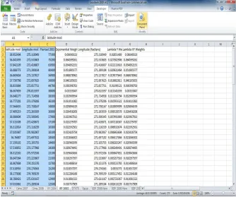
1.5 This ﬁgure shows the Excel spreadsheet with data. For this application to run properly, the ﬁrst row can contain any column names the reader wishes. Column 1 must contain the latitude observations. Column 2 must contain the longitude observations. Column 3 must contain the random variable of interest. It is not advisable to put any observations in the remaining columns as

this application may over-write them. 11

2.1 This ﬁgure shows the Map Point dialog box for ﬁnding a point on

the Earth using the latitude and longitude. 14

(15)

xiv LIST OF FIGURES

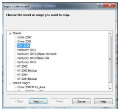
2.2 This figure shows the Map Point dialog box for browsing Excel files, which have the coordinates and the random variable. 15 2.3 This figure shows the Map Point dialog box that lists the Excel

spreadsheets in the Excel workbook. 15

2.4 This ﬁgure shows the Map Point dialog box containing the

spreadsheet column names and the data. 16

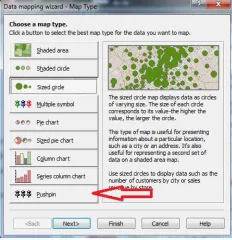
2.5 This ﬁgure shows the Map Point Data mapping wizard. 17

2.6 This figure shows the Map Point choices for the pushpin colors. 17 2.7 This figure shows the Map Point choice for the column chart. 17 2.8 This figure shows the Map Point choices for scaling the data and

change the label text. 18

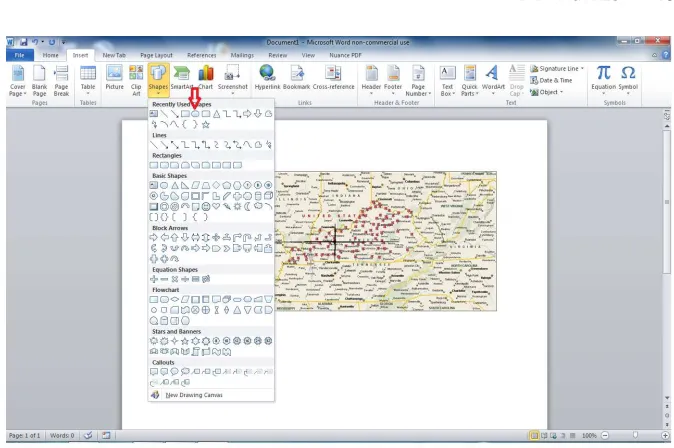
2.9 This ﬁgure shows the Microsoft Word shapes for drawing an

ellipse. 19

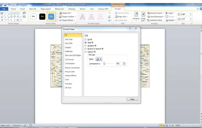
2.10 This ﬁgure shows the Microsoft Ofﬁce dialog box for formatting

a shape. 20

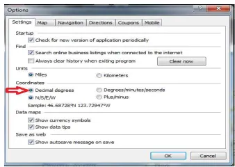
3.1 This ﬁgure shows theOptions dialog box in Map Point. We use it to convert the latitude and longitude coordinates to decimal

degrees. 28

3.2 This ﬁgure shows theOptions dialog box in Google Earth. We use it to convert the latitude and longitude coordinates to decimal

degrees. 28

3.3 This ﬁgure shows the Earth using Map Point. We identify points

on the Earth using latitude and longitude. 36

4.1 This ﬁgure shows Google Earth. It shows how to geo-code a

county with-in a state. 42

4.2 This ﬁgure shows the Excel spreadsheet of the Kentucky data. The spreadsheet has not been geo-coded. It still contains the

regional data. 44

4.3 This ﬁgure shows the Excel spreadsheet of the crime data. The spreadsheet has not been geo-coded and still contains the regional data, two years of data in the same spreadsheet, merged

columns, and percentages. 49

(16)

LIST OF FIGURES xv

5.1 This ﬁgure shows the Kentucky data from 2003 and the standard deviational ellipse. It shows a sketch of the standard deviational ellipse with Ohio County at the center. The semi-major axis is approximately 184 miles long and the semi-minor axis is approximately 52 miles long. We rotated the major axis roughly

70_{from the Y-axis in an imaginary Cartesian coordinate system.} ₆₆

5.2 This ﬁgure shows the standard deviational ellipse of violent crime in the US for the year 2007. It also shows the values of the violent crime using a bar graph. The ellipse is rather large

compared to the area in the survey. 69

5.3 This ﬁgure shows the plot of the mean center for the Air France

Flight 447 data. 70

5.4 This ﬁgure shows the plot of the mean center for the Malaysia

Flight MH 370 data. 71

5.5 This ﬁgure shows the plot of the mean centers of global GDP on a map. As the years progress, the mean center measurements

move closer to the Chinese coastline. 72

5.6 This ﬁgure shows the plot of the mean centers of global GDP on a map. As the years progress, the mean center measurements

move closer to the Greece coastline. 73

6.1 This ﬁgure shows the probability plot of the weighted latitude transformation. The exponential distribution ﬁts the weighted

latitude data since it shows a straight line. 84

6.2 This ﬁgure shows the probability plot of the weighted longitude transformation. The exponential distribution ﬁts the absolute value of the weighted longitude data since it shows a straight line. It was necessary to take absolute values since longitudinal

data is negative. 84

6.3 This ﬁgure shows sketches of both the standard deviational ellipse and the exponential deviational ellipse from the Kentucky data for the year 2003. The exponential ellipse is the smaller of the two ellipses. It covers one-third the area of the standard deviational ellipse, yet one-half of the same points. 93

6.4 This ﬁgure shows a raised bar graph of the weights in their respective counties for the Kentucky data for the year 2003. The majority of the weighted data comes from the lower-left corner of the state of Kentucky. The majority of the un-weighted data

(17)

xvi LIST OF FIGURES

6.5 This ﬁgure shows both the exponential deviational ellipse and the standard deviational ellipse for the violent crime data in the US for 2007. Both have the same center of gravity. The exponential ellipse is much smaller than the standard deviational ellipse. 95 7.1 This ﬁgure shows both the Weibull deviational ellipse for the

Kentucky data for the year 2003. The zoom level is 200 miles above the earth. The standard deviational ellipse and the exponential deviational ellipse were too large to ﬁt on the map. It has the same center of gravity as the other ellipses. The Weibull

ellipse is much smaller than the other two. 123

7.2 This ﬁgure shows both the Weibull deviational ellipse for the Crime data for the year 2007. The zoom level is 550 miles above the earth. The standard deviational ellipse was too large to ﬁt on the map. It has the same center of gravity as the other ellipses. The Weibull ellipse is much smaller than the other two. 124

8.1 This ﬁgure shows a map of the U.S. relative to the Equator

(represented by the black line). 141

8.2 This ﬁgure shows the diagram of a triangle with the quantities for the longitudeθ, n0,and the resultant lengthR. 146

8.3 This ﬁgure shows the histogram for the Kentucky 2003 data. 148

8.4 This ﬁgure shows the Kentucky 2003 converted data. 148

8.5 This ﬁgure shows the histogram for the Violent Crime 2008 data. Three possible modes appear at California, Texas, and Florida. 151

8.6 This ﬁgure shows the 2008 US Crime converted data. 151

8.7 This ﬁgure shows the plotted, unweighted data for Malaysia

Flight MH 370. 153

8.8 This ﬁgure shows the histogram for the GDP 2008 data. The U.S. accounts for approximately 25% of the total GDP and China

accounts for approximately 14%. 155

8.9 This ﬁgure shows the 2008 Gross Domestic Product converted

data. 155

A.1 In Excel, double click on the module named Ch4StandardDeviationalEllipse

on the left-hand pane circled in red to display the VBA code for the Standard Deviational Ellipse. The subroutine called Standard Dev Ellipse() runs the programs to calculate

(18)

LIST OF FIGURES xvii

A.2 This ﬁgure shows the VBA environment for the module named Ch4StandardDeviationalEllipse. It also highlights the driver

subroutineStandard Dev Ellipse(). 169

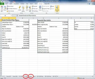
A.3 This ﬁgure shows theSTATS worksheet and the results from the Standard Dev Ellipse() subroutine. 170 B.1 This ﬁgure shows the VBA environment for the module

Ch5ExponentialDeviationalEllipse. It also

highlights the driver subroutineExponential Dev Ellipse(). 174

B.2 This ﬁgure shows theSTATS worksheet and the results from the Exponential Dev Ellipse() subroutine. 175 C.1 This ﬁgure shows the VBA environment for the moduleCh6

Weibull Deviational Ellipse. It also highlights

the driver subroutineWeibull Dev Ellipse(). 180

C.2 This ﬁgure shows theSTATS worksheet and the results from the

Weibull() subroutine. 182

D.1 This ﬁgure shows the VBA environment for the module

Ch7NewtonGaussRoutines. It also highlights the driver

(19)

(20)

LIST OF TABLES

3.1 Values of the Eccentricitye 31

3.2 Stratiﬁcation Deﬁnitions 34

3.3 Example of Estimation with Stratiﬁcation on Latitude 35 3.4 Example of Estimation with Stratiﬁcation on Longitude 35

4.1 Acreage Planted Data 46

4.2 Acreage Planted Data (con’t) 47

4.3 Acreage Planted Data (con’t) 48

4.4 Violent Crime Data 51

4.5 Violent Crime Data (con’t) 52

4.6 Air France Flight 447 Data 53

4.7 Malaysia MH 370 Data 54

4.8 Gross Domestic Product for OECD Countries 56

5.1 2003 Results on Corn acreage in Kentucky 67

(21)

xx LIST OF TABLES

5.2 2004 Results on Corn acreage in Kentucky 67

5.3 2007 Results on Violent Crime in the U.S. 68

5.4 2008 Results on Violent Crime in the U.S. 68

5.5 Results on Air France Flight 447 69

5.6 Results on Malaysia Flight 370 70

5.7 2008 Results on Gross Domestic Product of OECD Countries 71 5.8 2009 Results on Gross Domestic Product of OECD Countries 72 5.9 2008 Results on Gross Domestic Product of OECD Countries 73 5.10 2009 Results on Gross Domestic Product of OECD Countries 74 6.1 2003 Results for the Exponential Model for Kentucky 94 6.2 2004 Results for the Exponential Model for Kentucky 94 6.3 2007 Results for the Exponential Model on Violent Crime in the

U.S. 95

6.4 2008 Results for the Exponential Model on Violent Crime in the

U.S. 96

6.5 Results for the Exponential Model on Air France Flight 447 96 6.6 Results for the Exponential Model on Malaysia Flight MH 370 97 6.7 2008 Results for the Exponential Model on Gross Domestic Product 97 6.8 2009 Results for the Exponential Model on Gross Domestic Product 97 6.9 Relationship of angles of rotation for largex

is. 101

6.10 Relationship of angles of rotation for smallx

is. 101

(22)

LIST OF TABLES xxi

7.8 2009 Results for the Weibull Model on Gross Domestic Product 126

8.1 Interpretation of the Eigenvalues 146

(23)

(24)

FOREWORD

This book is a practical reference guide accompanied with an Excel Workbook. This book gives an elementary introduction of the weighted standard deviational ellipse. This book also presents the computational aspects of the weighted exponential distri-butions as well. For the examples given, calculations are performed using VBA for Excel. This book makes comparisons (and shows the computations via VBA for Ex-cel) using the likelihood functions with spatial data of the weighted ellipses. Lastly, the book covers spherical statistics. Throughout the text, the reader can see how to perform these difﬁcult calculations and learn to adapt the code for his research.

This book is a work in progress. Meaning,

Revising existing text. Modularizing source code.

Adding new text to existing text (e.g. new examples, new source code).

(25)

(26)

PREFACE

Scientific articles exist since the 1960’s for the use of an area frames for collecting and interpreting survey data in the United States, and in the 1990’s in Europe and Africa. Cartographers divide units of land from satellite imagery into enumerable segments. Statisticians assign the segments to defined strata. Typically, crop esti-mation is performed using imagery analyzes, field surveys, and mail surveys. The following list of articles includes both practical results and theoretical results typi-cally found in the literature on area frame surveys.

[Pratt, Bird, Taylor, and Carter (53)] wrote a paper that covers the topics of plan-ning and implementing an area frame survey in Nigeria and choosing the estimation procedures. They were careful to choose their satellite imagery and coordinate it with the fieldwork. In Europe and Africa, Statisticians use regression to classify the satellite images from field data collection and from image classification. Image classification without field data collection does tend to lead to failure due to the fol-lowing reasons: 1) intercropping practices, 2) fallow/cultivated continuum and 3) small, irregular field structure. The authors more generally state those reasons as ”spectral confusion.” The authors state that the best time to perform their fieldwork is shortly after harvest because it would be easiest to distinguish harvested rice fields from wet, green swamp grasslands. [page 70] calculates the sample size in terms of segments according to several criteria: 1) the size of the study size area, 2) the need to maximize the area covered, 3) the speed to cover the area during enumeration, 4)

(27)

xxvi PREFACE

reduce locational error within the segment during field mapping. The authors ob-tain a 4.8% sampling fraction by choosing forty-nine segments (500×500 meters with a sampling fraction of 5%) out of 75. Three estimators of the data collected are presented: 1) direct expansion of the survey data, 2) pixel count, and 3) regres-sion estimator. The authors recommend the regresregres-sion estimator, which take into, account both the irrigation mapped by enumerators on the ground in each segment and the satellite image classification. This is because it was highly dependent on the classifier and gave a narrower range of possible classifications. They used a ratio of the direct expansion variance and the regression model to prove this mathematically. [Kelly (33), Chhikara and Deng (7), Faulkenberry and Garoui, (16)] discuss area-frame data collection and estimation in the United States. [Kelly (33)] collects and summarizes survey data in a production environment. [Chhikara and Deng (7)] con-sider the problem of using the area frame and rotating segments amongst years. On page 926, they develop an ANOVA model to capture the stratum means per year and the segment mean effects for a particular random variable. The author also rotates and overlaps segments amongst years via a simulation study that shows the optimal rotation of segments should be 40% to 60%. [Faulkenberry and Garoui, (16)] discuss the topic of estimating population totals and variances from an area survey frame. The authors point out that because of the association of a farm with more than one segment does not lead to cluster sampling. Based on four classifications, the authors show that the Horvitz-Thompson estimator for totals is probably the best choice of estimators. It is a good estimator when the probability of selectionπkis proportional

with the random variablesy

ks.Depending on the number of farms or the number of

known segments, four classiﬁcations arise. The author assigns an estimator to each class that will work well, and then takes expectations and variances.

Although most of the authors so far do present maps with their articles and their statistical estimation methods, they lack discussing the latitude and longitude of their random variables. The remainder of this section will discuss the history of associat-ing random variables with the latitude and longitude (i.e. the placement on a map).

[Ebdon, (14), Chapter 7, 1985] discusses spatial statistics and several measures. The author gives interpretations to the concepts of the mean center and standard deviational ellipse. For instance, the mean center can be thought of the ”center of gravity” of the distribution of the given points on a map. He deﬁnes the standard deviational ellipse as the ”spread of points” about the mean center. Without using modern software, the author has an interesting way to draw the ellipse. It involves plotting the deviation for each point parallel to the rotated axes and ﬁtting the ellipse [Ebdon, (14), p. 137].

(28)

PREFACE xxvii

1. The center of the system determined by the distances from the central point (versus the extreme unit locations).

2. The direction or trend of the system given by the angleθmof the axis of

max-imum standard deviational variation value. This is the line of best ﬁt for the entire system of unit locations.

3. The concentration of the system (or dispersion) shown in terms of a standard deviational ellipse.

4. The relative concentration given by the ratio of observations within the ellipse compared to the entire population expressed in area units.

The author gives no references in the paper. To summarize, the article presents the mean and standard deviation of a set of numbers — longitude and latitude. So, who came up with the idea of weighting the longitude and latitude data?

The weighted standard deviational ellipse appears in the literature in 1971 in [Yuill, (68)]. The author begins with a discussion of the work by Lefever and the comments by Furtey in 1927. The paper proceeds to defend using the ellipse for geographic applications. The author derives the formulas on pages 30-31 for the weighted standard deviational ellipse. It is on page 32 that the weighted mean center is introduced (a new notion in the literature). The author weights the latitude and longitudinal observations using the random variable. The author gives the following computations for comparing ellipses.

1. The enclosed area within the ellipse.

2. The number of points enclosed within the ellipse (more is better). 3. The shape of the ellipse measured by its eccentricity .

The shape of the ellipse determines the distribution of the points . Points con-centrated at the pole of the ellipse (or circle) should have a non-uniform distribution while those scattered from the pole will have a uniform distribution . Finally, the au-thor applies the concepts to several sets of data. References appear in the footnotes throughout the paper.

(29)

xxviii PREFACE

according to the distribution of the phenomenon. If a city’s population is the ran-dom variable of interest, then the city’s population is the weight for the latitude and longitude. We apply weights in the context of [Lee and Wong, (37)] in this book.

(30)

ACKNOWLEDGMENTS

Map Point, Excel, and MS Word are products of Microsoft Corporation

Google Earth is a product of Google, Inc.

R. L. G.

(31)

(32)

ACRONYMS

GDP Gross Domestic Product

OECD Organization for Economic Cooperation and Development SDE Standard Deviational Ellipse

VBA Visual Basic for Applications

Random Variables, Their Properties, and Deviational Ellipses. By Roger L. Goodwin Copyright c2015 Roger L. Goodwin

(33)

(34)

CHAPTER 1 INTRODUCTION TO VBA

1.1 The Development Environment

The calculations in this book are difﬁcult at times. Having a programming environ-ment becomes advantageous. A programming environenviron-ment provides the ﬂexibility to calculate statistics and likelihood functions. This textbook uses the Visual Basic Application (VBA) for Excel. It is a programming environment based on the Visual Basic programming language. The VBA Development environment does not auto-matically appear as a menu option in Excel. See Figure 1.1. The user must make this option visible by following these steps:

1. Click onFile | Options | Customize Ribbon. The dialog box in Figure 1.2 will appear.

2. From theChoose Commands drop-down list, selectMain Tabs.

3. HighlightDeveloper.

4. Click on theAdd>> button in the middle of the screen.

(35)

2 INTRODUCTION TO VBA

Figure 1.1 This ﬁgure shows Excel without the Developer menu.

(36)

VARIABLES 3

Figure 1.3 This ﬁgure shows Excel with the Developer menu at the top of the screen.

TheDeveloper menu option will appear somewhere along the top of the screen. See Figure 1.3.

1.2 Variables

To declare variables explicitly in VBA for Excel, use the Dim statement. Excel supports the following basic data types:

Integer numbers —DimX As Integer The Integer data type holds integer variables stored as 2-byte whole numbers in the range of -32,768 to 32,767. Real numbers —DimYAs Double.TheRealdata type holds double-precision ﬂoating-point numbers as 64-bit numbers in the range of -1.79769313486231E308 to -4.94065645841247E-324 for negative values and 4.94065645841247E-324 to 1.79769313486232E308 for positive values.

String characters — DimS As String. The Stringdata can include letters, numbers, spaces, and punctuation. TheStringdata type can store ﬁxed-length strings ranging in length from 0 to approximately 63,000 characters.

(37)

Dates are stored as part of a real number. Values to the left of the decimal represent the date; values to the right of the decimal represent the time. Negative numbers represent dates prior to December 30, 1899.

A date can be any sequence of characters with a valid format surrounded by number signs (#). Valid formats include the date format speciﬁed by the locale settings for your code or the universal date format. For example, use #12/31/92# in the VBA editor when explicitly referring to a date.

Currency —DimQAs Currency. TheCurrency data type has a range of -922,337,203,685,477.5808 to 922,337,203,685,477.5807. Use this data type for calculations involving money and for ﬁxed-point calculations where accuracy is particularly important. In the VBA Editor, use the ”@” sign when referring to currency.

Long integer —DimR As Long. TheLongdata type is a 4-byte integer ranging in value from -2,147,483,648 to 2,147,483,647. In the VBA Editor, use the ”&” symbol when referring to long integers.

Logical —DimLAs Boolean. TheBooleandata type has only two possible values, True (-1) or False (0).

Variables defined inside a subroutine are visible only inside that subroutine. Vari-ables defined at the module level are visible to the subroutines defined in that module.

1.3 Arrays and Records

We can build on the basic data types listed in Section 1.2. Consider arrays and records.

One diminisional array —Dim Name List(1To 10) As String. This array deﬁnes a set of sequentially indexed elements having the data typeString.Each element of the array has a unique identifying index number. Changes made to one element of an array do not affect the other elements.

Two diminisional array —DimAList(1To5, 1To10)As Double. This array deﬁnes a matrix of indexed elements having the numeric data typeDouble.

(38)

BRANCHING 5

1              

TypeCustomers

3

        

First Name, Last NameAs String AddressAs String

CityAs String StateAs String Zip CodeAs Integer PhoneAs Integer End Type

2DimListAsCustomers

Do not use theDiminside theTYPE-END-TYPEstatement. Use the dot ”.” notation to reference the items in the record. For example in the VBA Editor, to reference the customer phone number, use the code:

1List.Phone = 3223223

1.4 Branching

VBA has anIF-THEN-ELSEstatement for conditionally executing code. The syn-tax is as follow:

1        

2



If<condition>Then VBA statements

3

  

Else

VBA statements End If

TheIF-THEN-ELSEconstruct must appear in a subroutine. It cannot appear as open code in a module. Aside from variable deﬁnitions and subroutine declarations, this is true for the majority of VBA programming. There can only by oneELSE

statement in anyIF-END-IFconstruct. An alternative to the aboveIF-THEN-ELSE

(39)

6 INTRODUCTION TO VBA 1                    2 

If<condition>Then VBA statements

3



ElseIf<condition>Then VBA statements

4



ElseIf<condition>Then VBA statements 5  Else VBA statements  End If

If the user has a short, single VBA statement for any of theELSEIFstatements, it is not advisable to put it on the same line after theTHEN. It usually creates a run-time error even though the syntax looks correct.

1.5 Loops

The two loops covered in this section are theFOR-NEXTloop and the WHILE-WENDloop. To execute a set of VBA statements a given number of times in a given sequence, theFOR-NEXTloop has the following syntax:

1   

For<counter>=startToend VBA statements

Next<counter>

As an example, we can generate two digits in a phone number.

1         

multiplier = 1 List.phone = 0

2     

Fori=1To 7

List.phone = List.phone + i*multiplier multiplier = multiplier * 10

Nexti

The value ofList.phone is 28 because n(n₂+1) = 7(8)₂ = 28.The only pur-pose of the example is to show the syntax of theFOR-NEXTloop.

TheWHILE-WENDloop has the following syntax.

1   

While<condition>

(40)

SETTING PROPERTIES 7

It is more likely to program inﬁnite loops with theWHILE-WENDloop than with theFOR-NEXT loop. It is important to initialize the condition variable(s) before entering the loop and to update the condition variable(s) inside the loop.

1.6 Setting Properties

Both the Excel spreadsheet and the VBA environment allow the user to change the cell contents properties to bold, italic, underline, strikethrough, and the font size. Except for the font size, most of these properties are Boolean valued.

Object.Bold — Boolean Object.Italic — Boolean Object.Size — Integer

Object.StrikeThrough — Boolean Object.Underline — Boolean

In our case, the VBA object is a cell in a spreadsheet. We use the following code to reference the properties of the cell.

1       

ActiveSheet.Cells(1, 3).Font.Bold = True ActiveSheet.Cells(1, 3).Font.Italic = True ActiveSheet.Cells(1, 3).Font.Size = 25

ActiveSheet.Cells(1, 3).Font.Strikethrough = True ActiveSheet.Cells(1, 3).Font.Underline = True

Cells(1,3) references row 1, column C in the last spreadsheet viewed before entering the VBA environment. Alternatively, we could have substituted the Ac-tiveSheet with a speciﬁc spreadsheet name such asWorksheets("Sheet1"). We have hard-codedSheet1. Sheet1 will always be the spreadsheet refer-enced.

When updating a set of cells in a spreadsheet, it is convenient to use the WITH-END-WITHstatement. It can save some typing and make the code easier to read. For example, we can re-write the VBA code for the font updates as follow:

1            

WithActiveSheet

.Cells(1, 3).Font.Bold = True .Cells(1, 3).Font.Italic = True .Cells(1, 3).Font.Size = 25

.Cells(1, 3).Font.Strikethrough = True .Cells(1, 3).Font.Underline = True End With

(41)

1.7 The Excel Examples

The Excel spreadsheet and the Excel VBA environment contain many of the same functions. Some common syntax and conventions for the worksheet follows.

1. Columns in an Excel worksheet always begin with a letter.

2. Rows in an Excel worksheet always begin with a number.

3. The three default names of the worksheets in an Excel workbook areSheet1, Sheet2, andSheet3. Microsoft Corporation capitalized the ”S” in the word ”Sheet.” In the VBA for Excel environment, upper and lower case counts.

4. Character and numeric data can ordinarily be copy and pasted into the work-sheet cells.

5. Precede numeric data with leading zeros with the single quote ” ’ ”to retain those leading zeros. Entering the single quote in front of the data is a man-ual operation. Changing the column to the TEXT format usman-ually causes other problems later on.

6. Formulas begin with an equal sign. Some useful formulas used in this applica-tion include:

mod(number, divisor) — where the argumentnumber can either be reference to a cell or a hard coded number such as 180 or 360; and the argumentdivisor can either be a cell reference or a hard coded number such as 180 or 360.

average(range) — where the argument range is a range of cells such asA2..A91.

sum(range) — where the argumentrange is a range of cells such as C2..C39.

In this application, we keep the data and results in the worksheets. We use VBA to perform the calculations. Some common conventions in VBA for Excel follow.

1. Declare global variables at the top of a module.

2. VBA program code must appear inside a subroutine. Some useful, recurring VBA statements used in this application include:

(42)

THE EXCEL EXAMPLES 9

ActiveSheet.Cells(row, col).Value —

The activesheet object references the data in the spreadsheet high-lighted before entering the VBA editor. This entire statement allows reading the data.

Worksheets("name").Cells(row, col).Value —

Theworksheets object references the spreadsheet namedNAME. In the application name = stats. This entire statement allows writing data to a spreadsheet other than the active spreadsheet.

For-Next — This is the common looping structure used for calculating the sums, the areas, the probability distributions, eccentricities, and so on. While-Wend This application uses this looping in Module 3 in the Secant algorithms because the termination condition required more knowledge that the number of observations in the data set.

VBA numeric calculations — The Visual Basic for Excel numeric calcula-tions are similar in style to those of other programming language statements.

Some useful, recurring VBA functions used in this application include:

log(number) — This function returns the latural logarithm of the given number. The user must write his own code for other base logarithms. exp(number) — This function returns the exponential function of the givennumber. eis approximately 2.718282.

worksheetfunction.pi() — This function returns the value ofπ.

3. Modules are a collection of related subroutines and variables. 4. Declare local variables inside a subroutine.

5. Variable names are not case sensitive. For all declared variables, the VBA editor will change the upper and lower case spelling.

In this application, the results are stored in the spreadsheet called STATS. See Figure 1.4. The data are stored in the remaining spreadsheets. The ﬁrst three columns of the data must be in a particular order. Seel Figure 1.5.

1. Latitudexi.

2. Longitudeyi.

3. Random variable of interestwi.

Further, select the data (and only the data) so that the subroutines can identify the beginning and ending rows. To get into the VBA editor, follow these steps.

(43)

[image:43.612.76.409.245.522.2]

(44)

[image:44.612.75.409.235.514.2]

THE EXCEL EXAMPLES 11

(45)

2. Click on theVisual Basic button on the left side.

3. For a new module, click on theInsert menu item and select Module.

(46)

CHAPTER 2 INTRODUCTION TO MAP POINT

Map Point is a software package that maps points on the Earth. The user provides the latitude and longitude, and Map Point plots the point. The points in this textbook are either geo-coded observations from Google Earth or calculations such as the mean center (also called the center of gravity) or the semi-major and semi-minor axis lengths of an ellipse. It is possible to enter, say a county name into Map Point. Map Point will identify the county on the Earth. However, it will not give the user the latitude and longitude coordinates. This is why we must use an alternate software product.

There are several useful concepts when using Map Point:

1. Plotting the mean center on the Earth.

2. Plotting and graphing the entire survey of points on the Earth.

3. Drawing lines with an exact length in miles (or kilometers).

4. Saving work.

5. Copying and pasting images to other software applications.

(47)

14 INTRODUCTION TO MAP POINT

Figure 2.1 This ﬁgure shows the Map Point dialog box for ﬁnding a point on the Earth using the latitude and longitude.

Map Point does allow us to draw ellipses. However, it does not allow us to rotate them. Because of this, we must draw ellipses outside of Map Point. We use Map Point to draw the semi-major axis and the semi-minor axes.

2.1 User Data

Map Point has two ways to enter data:

1. Manually one data point at a time usingTools | Find | Lat\Long. 2. Import an Excel spreadsheet usingData | Data import wizard.

When the user enters data manually, one data point at a time, Map Point requests the latitude and the longitude. When the user imports multiple data points via an Ex-cel spreadsheet, Map Point requires column names with ”latitude” and ”longitude.” In addition, Map Point expects the user to plot a third variable called a ”data” vari-able or an analysis varivari-able along with the latitude and longitude. Naming the third variable is at the user’s discretion. Notes on entering data manually appear in Section 2.2. More notes follow on importing data in Section 2.3.

2.2 Plotting the Mean Center

(48)

[image:48.612.182.303.299.413.2]

VISUALIZING THE SURVEY DATA 15

Figure 2.2 This ﬁgure shows the Map Point dialog box for browsing Excel ﬁles, which have the coordinates and the random variable.

Figure 2.3 This ﬁgure shows the Map Point dialog box that lists the Excel spreadsheets in the Excel workbook.

at the top of the dialog box, the user types in the coordinates and clicks on theFind button. Map Point will locate that latitude and longitude on the Earth and identify those coordinates with a box.

2.3 Visualizing the Survey Data

Sometimes the user may want to visualize the survey data (i.e. many data points) and the ellipse together (i.e. drawing). Alternatively, maybe, the user may want to visu-alize the plotted points on the Earth with the random measurements (i.e. graphing). Map Point does provide the software tool to plot or graph an entire data set onto the Earth.

(49)

Figure 2.4 This ﬁgure shows the Map Point dialog box containing the spreadsheet column names and the data.

The dialog box in Figure 2.2 allows the user to browse the hard drive and select the Excel ﬁle that contains the survey data.

Map Point displays the dialog box in Figure 2.3 showing the spreadsheet names in the Excel workbook. Select one of the spreadsheets.

Click theNext button in the Import Data Wizard. The screen in Figure 2.4 appears showing the columns and the data in the spreadsheet.

Click theFinish button.

TheData mapping wizard in Figure 2.5 appears. There are some choices here. Do we want to use shaded circles, sized circles or pushpins to mark the points on the Earth? The remaining options pertain to graphing the data. We will discuss graphing later. Let us choose pushpins since they stand out the best.

Click on thePushpin button.

Click on theNext button at the bottom of the dialog box. The dialog box in Figure 2.6 appears. The user can change the color of the pushpins here, if desired. Map Point automatically recognized the column nameslatitude andlongitude. This is important because the user would have had to identify these had this not been the case.

(50)

VISUALIZING THE SURVEY DATA 17

Figure 2.5 This ﬁgure shows the Map Point Data mapping wizard.

[image:50.612.184.300.145.265.2]

Figure 2.6 This ﬁgure shows the Map Point choices for the pushpin colors.

(51)

[image:51.612.182.302.129.254.2]

Figure 2.8 This ﬁgure shows the Map Point choices for scaling the data and change the label text.

2.3.0.2 Graphing To graph the data, first prepare an Excel file with the survey data. Save the Excel file to the hard drive. SelectData | Import data wiz-ard.

The dialog box in Figure 2.2 allows the user to browse the hard drive and select the Excel ﬁle that contains the data to analyze.

Map Point displays the dialog box in Figure 2.3 showing the spreadsheet names in the Excel workbook. Select one of the spreadsheets.

Click theNext button in the Import Data Wizard. The screen in Figure 2.4 appears which shows the column names and the data.

Click theFinish button.

TheData mapping wizard in Figure 2.5 appears. There are some choices here. Do we want our data displayed as a pie chart, sized pie chart, column chart, or as a series column chart? The remaining options pertain to plotting the data. We discussed plotting data in the previous section.

Click on theColumn chart button.

Click on theNext button at the bottom of the dialog box. The dialog box in Figure 2.7 appears. Map Point automatically recognized the column names latitude andlongitude. The user must conﬁrm to Map Point to graph the column name2008.

(52)

[image:52.612.73.410.113.337.2]

DRAWING AXES 19

Figure 2.9 This ﬁgure shows the Microsoft Word shapes for drawing an ellipse.

bars represent large values. Map Point places the bars on the Earth using the latitude and longitude coordinates.

2.4 Drawing Axes

Before drawing an axis, it may be necessary to zoom into the survey area. To draw an axis for an ellipse which has an exact length measured in miles or kilometers, selectTools | Measure distance. To toggle between miles and kilo-meters, selectTools | Options and the dialog box in Figure 3.1 will appear. The section onUnits changes the unit of measure.

Single click on the label box for the mean center. This will anchor the ruler. Map Point displays the unit of measure and number of measurements at the right side of the line.

Drag the mouse the length required.

Single click. This will anchor the right end of the line. Hit the<Esc>key to stop drawing lines.

2.5 Drawing Ellipse Boundaries

(53)

[image:53.612.77.408.126.335.2]

Figure 2.10 This ﬁgure shows the Microsoft Ofﬁce dialog box for formatting a shape.

Draw the axes described in Section 2.4 using an imaginaryXandY-axes laid on top of the Earth.

Note the axis of rotation (e.g.XorY)from the statistical computations.

Copy and paste the image from Map Point into MS Word. The imaginaryX

andY-axes form90_{angles. Half of}₉₀_is₄₅_,_{and so on. If the rotation is}

from theY-axis, then begin counting from there.

In MS Word, selectInsert | Shapes. The shapes in Figure 2.9 will appear.

Select the ﬁfth shape from the top,oval. Left click and right click around the axes lengths. The oval will be dark ﬁlled.

Right click the oval. Left click the oval and selectFormat shape. The dialog box in Figure 2.10 will appear.

Click on theNo fill radio button.

Click onClose.

We drew the ellipse following the steps above. We need to rotate the ellipse. Suppose we want to rotate the ellipse from theY-axis70_._{Then, follow these steps:}

(54)

PROGRAMMER NOTES 21

A green circle appears at the top of the ellipse. This is for rotating the ellipse. Single click on the green circle.

Drag the mouse to obtain a70_{angle between the}_Y_{-axis and the semi-major}

axis. Certainly you know where90_and₄₅_{are at. This is not difﬁcult.}

SelectFile | Save As to save the ellipse.

To avoid the appearance ofcross hairs in any published graphs, the user can alternatively identify the ends of the major and minor axes using pushpins or some other symbol. When in Map Point, delete any lines drawn when using the ruler.

2.6 Programmer Notes

Microsoft Corporation did not provide Map Point with a development environ-ment as they did with Excel and MS Word. We need to perform repetitive re-search manually. The one advantage is that the registered version of Map Point does accept Excel ﬁles for plotting and graphing data.

Not being able to rotate ellipses in Map Point is a draw back. This is just another reason to leave Map Point for another software product.

(55)

(56)

CHAPTER 3 MATHEMATICS REVIEW

3.1 Notation

We discuss some common notation used throughout this book here.

(57)

24 MATHEMATICS REVIEW

Notation Meaning

x Subscript denoting latitude.

y Subscript denoting longitude.

t A dummy variable used in integration. Usually denotes the latitude.

u A dummy variable used in integration. Usually denotes the longitude.

w Subscript denoting the weight variable.

γx Shape parameter to the Weibull distribution for the latitude.

γy Shape parameter to the Weibull distribution for the longi-tude.

λx Scale parameter to the Exponential distribution and the Weibull distribution for the latitude. Generally, there is no implied equality.

λy Scale parameter to the Exponential distribution and the Weibull distribution for the longitude. Generally, there is no implied equality.

k The iteration number in the Secant algorithm.

n Denotes the sample size .

φi Represents the observed values of the latitude in spherical statistics.

θi Represents the observed values of the longitude in spherical statistics.

R Called the resultant length in spherical statistics.

¯

l0,m¯0,n¯0 Called the mean direction of cosines in spherical statistics.

S∗

Denotes the spherical variance.

T Denotes the matrix T.The diagonal elements sum to the

sample sizen.

B Denotes the matrixB.The diagonal elements sum to2n.

The set_{x1, x2, ..., xn}represents the observed values of the latitude. The set

{y1, y2, ..., yn}represents the observed values of the longitude. The set{w1, w2, ..., wn}represents the observed values of the random variable at those corresponding

latitude and longitude. Using these three sets of observed numbers(wi, xi, yi),we

estimate parameters from known distributions.

3.2 Derivatives

(58)

INTEGRALS 25

Example 1:

d(a)

dx = 0.

Example 2:

dlogen

dx = 0.

Example 3:

dlogeu

d x =

1

u du dx.

Example 4:

d eu

dx =e

udu

dx.

Take the derivative off(w, λ, x) =w_λ1e−x

λ with respect tox.

d w1_λe−x λ

d x =−w

₁

λ

2 e−x

λ

Example 5:

d xa

da =x

a_log_x.

We are not asking for the derivative with respect toxin this example.

3.3 Integrals

Some common integrals used in this text are given in this section.

Example 6:

 x

0

a du=ax.

Example 7: _

a

0

lnn dx=xlnn

   

a

0

=alnn.

Example 8:

 ₁

xdx= logx

Example 9:



eax=eax/a

(59)

3.4 Quadratic Equation

Most of the material in this section appears in CRC’s Standard Math Tables. A quadratic equation has the formax2₊_bx₊_c_{= 0}_._{Then, the roots are}

x=−b±

√

b2₋₄_ac 2a

Ifa, b,andcare real, then

1. Ifb2₋₄_ac_{is positive, then the roots are real and unequal.}

2. Ifb2₋₄_ac_{is zero, then the roots are real and equal.}

3. Ifb2₋₄_ac_{is negative, then the roots are imaginary and unequal.}

The roots to the quadratic equation give the equation for the standard deviational ellipse. Cases (1) and (2) have more practicable importance than (3). We will discuss the standard deviational ellipse and other ellipses in later Chapters.

3.5 Ellipse Equation

The elliptical formula appears in Equation (3.1).

(x−h)2

a2 +

(y−k)2

b2 = 1, a > b >0 (3.1)

It may be necessary to complete the quadratic equations in the numerators to obtain an ellipse.

3.6 Trigonometry Functions and Conversion Factors

In Excel, theAtn() function is used to obtain the argument xfrom the tangent functionT an(x).The function takes degrees as input, but returns radians as output. Given that, it is convenient to know the following conversion factors:

To convert radians to degrees,

1radian = 180

π = 57.2957795degrees.

To convert degrees to radians,

1degree = π

(60)

MODULO ARITHMETIC 27

3.7 Modulo Arithmetic

Modulo arithmetic arises when we convert spherical data to directional data. The spherical data comes from the observed latitude and longitude for a random event. To apply some statistical techniques, we need to convert the longitude to a circu-lar reference system, which results in directional data. To accomplish this, we use modulo arithmetic.

To convert the latitude coordinatesxi to the circular reference systemxiwe use

the general rule:

x

i=mod(xi,180). (3.2)

To convert the summary statistic for the mean latitudex¯back to the original co-ordinate system, we use the general rule:

¯

x₌



¯

x, ifx¯≤90_.

−mod(180,x¯), ifx >¯ 90_. (3.3)

The reader should not worry about how to calulatex¯in this Chapter. Realize that when samples with mixed signs for the latitude and longitude arise, we must have a mechanism to determine the sign of the summary statistics.

Example 10: The coordinates of Australia are (xi, yi) = (25 16 27.84 South,

133₄₆ ₃₀_.₄₉_East)_._{The decimal degree coodinates are}₍_x_i_{, y}_i_{) = (}₋₂₅_.₄₇₃₉₉_,

133.775136).

To convert the coordinates to decimal degrees in Map Point or Google Earth:

SelectTools | Options.

If using Map Point, the dialog box in Figure 3.1 will appear. If using Google Earth, the dialog box in Figure 3.2 will appear.

Click on the radion buttonDecimal degrees.

The latitude is negative. The longitude is positive. We convert the latitude using modulo arithmetic. The new latitude observation becomesx

i=mod(−25.47399,

180) = 154.52601.For computation purposes, we use the coodinates (xi, yi) =

(154.52601, 133.775136).

To convert the longitude coordinatesyito the circular reference systemyiwe use

the general rule:

yi=mod(yi,360). (3.4)

To convert the summary statistic for the mean longitudey¯back to the original coordinate system, we use the general rule:

¯

y= 

¯

y, ify¯≤180_.

(61)

[image:61.612.145.314.128.248.2]

Figure 3.1 This ﬁgure shows theOptions dialog box in Map Point. We use it to convert the latitude and longitude coordinates to decimal degrees.

Figure 3.2 This ﬁgure shows the Options dialog box in Google Earth. We use it to convert the latitude and longitude coordinates to decimal degrees.

Example 11:The coordinates of Canada are(xi, yi) = (55 56 18.59 North,106

20₄₈_.₃₇ _West)_._{The decimal degree coodinates are}₍_x

i, yi) = (55.938497,−106.

346771).The longitude is negative. The latitude is positive. We convert the longitude using modulo arithmetic. The new longitude becomesy

i=mod(−106.346771,360)

= 253.653229.For computation purposes, we use the coodinates (xi, yi) = (55.

938497, 253.653229).

3.8 Weighted Data

(62)

WEIGHTED DATA 29

level of geography reported by the BJS in the survey is at the state level. To ﬁnd the center of gravity of violent crime, we take the average of the latitude observations and the average of the longitude observations. Averages are un-biased estimators. To say that each state contributes equally to the center of gravity is misleading. Some states have a high number of incidents of crime while others have a low number of incidents of crime. We should reﬂect this fact in the estimator. The literature on weighted data typically multiplies the latitude and longitude by a weight. In this case, the weight is the number of incidents of violent crime divided by the sum of the number of incidents of violent crime for the entire U.S. This ensures the weights are between zero and one. It ensures those states with a high number of incidents of violent crime will have a correspondingly proportional effect on the center of gravity — those states will draw the mean center of gravity to themselves. Vise-versa, those states with a low number of incidents of violent crime will have the mean center of gravity pulled away from them.

Throughout the textbook, the examples use weighted data. Equation (3.6) shows the weighting scheme for observationiout ofnobservations.

w

i=

wi

n i=1wi

(3.6) 1                                 

SubSet Weights(sum weight)

’this procedure calculates the weights between 0 and 1 in column D ’columns A, B, and C must be highlighed

n =Selection.Rows.Count sum weight = 0

2       

Fori = 2Ton

4

  

WithActiveSheet

sum weight = sum weight +.Cells(i, 3).Value End With Next 3       

Fori = 2Ton

5

  

WithActiveSheet

.Cells(i, 4).Value=.Cells(i, 3).Value/ sum weight End With

Next End Sub

(63)

and stores the results in Column D. We do not weight observation i equal to 1 (i.e. row 1 in the active spreadsheet) because it is a label.

Upon running this subroutine, columnD will always sum to one. The use of the WITH-END-WITH statement is optional. It is a short-cut to not having to keep typ-ing in the Excel object — in this case, the spreadsheet last referenced ”Activesheet.”

3.9 Area

Consider the simple formula for calculating the area of an ellipse (or a circle). Let

abe the length of the semi-major axis. Letbbe the length of the semi-minor axis. Ifa > b,then we have an ellipse. Ifa = b,then we have a circle. A function to calculate the area of an ellipse is given next. The parameters to the function are the semi-major axis lengthaand the semi-minor axis lengthb.Equation (3.7) gives the formula for the area of an ellipse.

f =πab. (3.7)

1        

FunctionArea(a, b) ’a= semi-major axis length ’b= semi-minor axis length

2Area =WorksheetFunction.Pi* a * b End Function

Line 2 calculates the area of the ellipse using the formula in Equation (3.7). The value of the calculation is returned via the function nameArea.

3.10 Eccentricity

Equation (3.8) gives the eccentricity of an ellipse (or circle) whereais the length of the semi-major axis andbis the length of the semi-minor axis,a≥b.

e=

√ a2₋_b2

a (3.8)

1                

FunctionEccentricity(a, b) ’a= semi-major axis length ’b= semi-minor axis length

2

      

Ifa>=bThen

Eccentricity =Sqr(aˆ2 - bˆ2) / a ’ eccentricity Else

Eccentricity =Sqr(bˆ2 - aˆ2) / b ’eccentricity End If

(64)

AXES LENGTH 31

Some defensive programming has been incorporated into theEccentricity() function. Ifais the semi-major axis, then Equation (3.8) works ﬁne. If the user for-gets the variable deﬁnitions, then the function would return an error message if only one formula was programmed. Ifa < b,the roles ofaandbare switched in Equation (3.8). TheIF-THEN-ELSE statment (2) demonstrates the defensive programming concept.

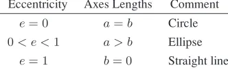
[image:64.612.148.314.282.333.2]

Table 3.1 summarizes the values of the eccentricity e and the accompanying shapes.

Table 3.1 Values of the Eccentricitye

Eccentricity Axes Lengths Comment

e= 0 a=b Circle

0< e <1 a > b Ellipse

e= 1 b= 0 Straight line

3.11 Axes Length

Equation (3.9) gives the formula for the semi-major axis lengtha.Equation (3.10) gives the formula for the semi-minor axis lengthb.

Calculating the valuesx, y,andxyare complicated sums depending on the proba-bility distribution. We will cover the details on calculating the sums in later Chapters. For now, assume that the variablesx, y,andxyare given.

Given the quantitiesx, y, xy, the subroutineAxes Length() returns the length of the semi-major axisaand the length of the semi-minor axisb.

a=   

_ny + 2(xy) 2

n−(x−y) +(x−y)2_{+ 4(}_xy₎2 (3.9)

b=   

_nx+ 2(xy) 2

(65)

1                              

SubAxes Length(m, x, y, xy, a, b) ’m= number of observations

’x= sum of diffs from mean center squared x direction (input) ’y= sum of diffs from mean center squared y direction (input) ’xy= diff sums from mean centers x and y direction (input) ’a= semi-major axis (output)

’b= semi-minor axis (output)

2

           

Ifx>=yThen

a =Sqr(y / m + 2 * (xy)ˆ2 / (m * (-1 * (x - y) +Sqr((x - y)ˆ2 + 4 * xyˆ2)))) b =Sqr(x / m - 2 * (xy)ˆ2 / (m * (-1 * (x - y) +Sqr((x - y)ˆ2 + 4 * xyˆ2)))) Else

a =Sqr(x / m + 2 * (xy)ˆ2 / (m * (-1 * (y - x) +Sqr((y - x)ˆ2 + 4 * xyˆ2)))) b =Sqr(y / m - 2 * (xy)ˆ2 / (m * (-1 * (y - x) +Sqr((y - x)ˆ2 + 4 * xyˆ2)))) End If

End Sub

3.12 Rotation

The subroutineAngle of Rotation() calculates the angle of rotationθin Equa-tion (5.10). It also gives the axis of rotaEqua-tion. The ﬁrst four VBA statements calculate the angle of rotation with the plus and minus sign accounted for. The angle of rotation

(66)

BASE 10 LOGARITHM 33 1                                                

SubAngle of Rotation(x, y, xy, note, atheta, itheta) ’calculate the rotation from the axes

’x= sum of diffs from mean center squared x direction (input) ’y= sum of diffs from mean center squared y direction (input) ’xy= diff sums from mean centers x and y direction (input) ’note= states direction of rotation (output)

’atheta= angle of rotation in the x direction (output) ’itheta= angle of rotation in the y direction (output)

tan theta1 = -1 * (x - y) / (2 * xy) +Sqr((x - y)ˆ2 + 4 * xyˆ2) / (2 * xy) tan theta2 = -1 * (x - y) / (2 * xy) -Sqr((x - y)ˆ2 + 4 * xyˆ2) / (2 * xy) theta1 =Atn(tan theta1) * 180 /WorksheetFunction.Pi()

theta2 =Atn(tan theta2) * 180 /WorksheetFunction.Pi()

2                

Iftheta1>theta2Then note = ”Rotate on Y-Axis” atheta = theta1

itheta = theta2 Else

note = ”Rotate on X-Axis” atheta = theta2

itheta = theta1 End If End Sub

3.13 Base 10 Logarithm

The VBA logarithm function has a natural exponential base. VBA for Excel does not provide a means to change the base of the logarithm. If the programmer wishes to change the base, then the programmer must write a function for that particular logarithm with that particular base. The static functionLog10(X) returns the log-arithm of the numberXwith the base 10.

1   

Static FunctionLog10(X) Log10 =Log(X) /Log(10#) End Function

3.14 Stratiﬁcation

(67)

the Weibull model, the latitude and the longitude must be positive. The OECD exam-ple in Section 4.4 is the ﬁrst examexam-ple to contain the full range of data. The other data sets contained mixed data where either the latitude had a full range−90≤xi ≤90

or the longitude had a full range−180≤yi ≤180,but never in the same data set.

For this reason, we must define strata for the exponential model and the Weibull model to return the same results as the regression model. An estimator will combine the strata estimates into a single estimate. Table 3.2 gives the strata definitions for the OECD data. The definitions work for both the latitude and longitude calcula-tions. The reader will have to separate the data, as the software does not give strata estimates directly.

Table 3.2 Stratiﬁcation Deﬁnitions Latitude Longitude Stratum

+ + 1

− + 2

+ − 3

− − 4

3.14.1 Latitude Estimates

The procedure for creating a latitude estimate for the exponential model and the Weibull model is as follow:

1. Stratify the data based on sign. This creates four strata. See Table 3.2. 2. Calculate stratum averages.

3. Combine stratum averages for latitude by:

(a) Stratum 1 and 3 latitude average givesx¯1,3. (b) Stratum 2 and 4 abs(latitude) average givesx¯2,4.

(c) Multiply the averages by the number of observations_ niin each strata where n

i=1ni=n.

(d) Average nix¯1,3+n



ix¯2,4

n .Note the average of the difference (the sign is

nega-tive for strata 2,4).

Example 12:Consider the example in Table 3.3. It shows how to obtain a consistent estimate when the signs change for the latitude. This example also accounts for unequal sample sizes in each stratum. x¯ = −2.65is incorrect because it assumes equal sample sizes in the strata. To obtainx¯=−0.34,

¯

x=9×8.9 + 6× −14.2

(68)

STRATIFICATION 35

Table 3.3 Example of Estimation with Stratiﬁcation on Latitude

Estimate ni Regression Exp Weibull Comment

¯

x1,3 9 8.9 8.9 8.9 Latitude strata 1,3 always positive

¯

x2,4 6 -14.2 14.2 14.2 Latitude strata 2,4 always negative

¯

x 15 -0.34 -0.34 -0.34

3.14.2 Longitude Estimates

The procedure for creating a longitude estimate for the exponential model and the Weibull model is as follow:

1. Stratify the data based on sign. This creates four strata. See Table 3.2.

2. Calculate stratum averages.

3. Combine stratum averages for longitude by:

(a) Stratum 1 and 2 longitude average givesy¯1,2. (b) Stratum 3 and 4 abs(longitude) average givesy¯3,4.

(c) Multiply the averages by the number of observations_ niin each strata where n

i=1ni=n.

(d) Average niy¯1,2+n



iy¯3,4

n .Note the average of the difference (the sign is

nega-tive for strata 3,4).

Example 13: Consider the example in Table 3.4. It shows how to obtain a consis-tent estimate when the signs change for the longitude. The answer¯y = 40.775is incorrect. That answer assumes equal stratum sizes. The correct longitude estimate is

¯

y =9×102.3 + 6× −20.75

15 = 53.08

Table 3.4 Example of Estimation with Stratiﬁcation on Longitude

Estimate ni Regression Exp Weibull Comment

¯

y1,2 9 102.3 102.3 102.3 Longitude strata 1,2 always positive

¯

y3_,4 6 -20.75 20.75 20.75 Longitude strata 3,4 always negative

¯

(69)

3.15 Coordinate Systems

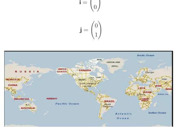
The Cartesian coordinate system is the classical coordinate system taught in most textbooks. In two dimensions, we have an X-axis and aY-axis. This is a single pole coordinate system with(0,0)at the center. In three dimensions, we have the additionalZ-axis — still a single pole coordinate system.

We can alternatively deﬁne the functionr = ix+jy,whereiandjare vectors deﬁned as:

i= 

1 0 

and

j= 

[image:69.612.94.381.238.448.2]

0 1 

Figure 3.3 This ﬁgure shows the Earth using Map Point. We identify points on the Earth using latitude and longitude.

In the spherical statistics literature, a one-pole coordinate system appears most often because these coordinate systems have the most practical applications and in-terpretations. Suppose we are measuring the hands on a clock, a roulette wheel, an experiment where a person in a room must identify the source of a sound, and so on. All of these examples have one common theme in that they have one pole. The center of the clock is the pole. The center of the roulette wheel is the pole. The person’s head is the pole. [Leong and Carlile (39)] describe thehoopcoordinate sys-tem, which has two dimensions and one pole. They mention that data is restricted to observations lying on the sphere as opposed to measuring distance (i.e. the sound experiment).

(70)

TESTING FOR RANDOMNESS 37

Another set of practicable problems use latitude and longitude coordinates. We identify points on the Earth using latitude and longitude. See Figure 3.3. We look-up the latitude and longitude coordinates for our data. This is calledgeo-coding.

The latitude ranges from(−90_,₉₀₎_._{The longitude ranges from}₍₋₁₈₀_,₁₈₀₎_.

We can always convert geographic data to circular data. The mean results can be converted back to the original coordinate system while preserving the sign. We must interpret the results such as the mean center, which is also called thecenter of gravity.

Using the calculations from the spherical statistics literature, these calculations strive to project the data onto an X, Y andZ-axis as opposed to the Earth. Using the calculations from the geography and statistics literature, the center of gravity will always be in the survey area. Some careful forethought goes into what you expect from spherical statistics.

Many times the data in this textbook comes from several sources. The random variablewi augments with a pair of coordinates called latitudexi and longitude

yi for each observationi. We omit the altitude from the analysis. Using special

software, we plot the random variable on a map using the pair(xi, yi). To make

calculations simple, we measure the latitude and longitude pairs(xi, yi)indegrees,

thendecimal minutes and seconds as opposed to degrees, minutes, and seconds. Having knowledge of the Cartesian coordinate system for plotting points does help to understand the subtle differences between mapping and plotting.

When drawing an ellipse on a map, knowledge of the polar coordinate system is most useful. We derive several pieces of information:

The center of the ellipse.

The semi-major and the semi-minor axis lengths. The angle of rotation from an imaginaryXorY-axis.

We have enough information to draw an ellipse and to rotate the ellipse from the imaginary axis. The imaginary axis (or axes) is simply theX andY-axes from the Cartesian coordinate system super-imposed onto a map using specialty software. Chapter 2 discusses some of the specialty software available.

The software comes with a ruler to draw lines. The software can measure lines in miles or kilometers. We use the ruler to draw the semi-major and semi-minor axes.

The user must use another software product to draw and rotate the ellipse.

3.16 Testing for Randomness