Time Varying Volatility Modeling of Pakistani and leading foreign stock markets

Munich Personal RePEc Archive

Time Varying Volatility Modeling of

Pakistani and leading foreign stock

markets

Ghouse, Ghulam and Khan, Saud Ahmed and Arshad,

Muhammad

Pakistan Institute of Development Economics, Islamabad, Pakistan

Institute of Development Economics, Islamabad, Govt. Commerce

College, Faisalabad

30 December 2015

Time Varying Volatility Modeling of Pakistani and leading foreign stock

markets

Ghulam Ghouse1

Pakistan Institute of Development Economics, Islamabad

PhD (Econometrics) scholar

Saud Ahmed Khan2

Pakistan Institute of Development Economics, Islamabad

Assistant Professor, Dept. Econometrics

Muhammad Arshad3

Govt. Commerce College, Faisalabad

Lecturer, Dept. Economics

Abstract

This study estimates the volatility of Pakistani and leading foreign stock markets. Daily data are

used from nine international equity markets (KSE 100, NIKKEI 225, HIS, S&P 500, NASDAQ

100, DOW JONES, GADXI, FTSE 350 and DFMGI) for the period of Jan, 2005 to Nov, 2014.

The whole data set is used for modeling of time varying volatility of stock markets. Univariate

GARCH type models i.e. GARCH and GJR are employed for volatility modeling of Pakistani and

leading foreign stock markets. The residual analysis also employed to check the validity of

models. Our study brings important conclusions for financial institutions, portfolio managers,

market players and academician to diagnose the nature and level of linkages between the

financial markets.

1. Introduction

Volatility modeling is one of the leading issue now a days addressed by financial econometrics.

Predictability of time varying volatility is the elementary purpose of financial econometric

modeling. In financial markets risk is a synonym of volatility. The understanding and

predictability of time varying volatility modeling is significantly important for asset allocation,

strategies of global hedging and pricing of internal securities. In econometrics the main purpose

of modeling of time series is to estimate the conditional mean, some theoretical models are used

to estimate conditional variance, it is also known as volatility. These models are employed to

analyze the historical behavior of volatility, future prediction of volatility, examining series of

asset return by considering volatility clustering, leverage effect and persistence. The volatility

clustering are piles of low and high values of financial asset return. The volatility clustering is

commonly seen in financial time series. The persistence of shock is a measure to demonstrate

how much time a price shock takes for decay in financial time series. Leverage effect illustrates

the negative correlation between current asset return and future volatility of asset return. All this

information can be obliging in portfolio allocation and hedging.

2. Literature review

This section briefly discusses previous studies. There’s a long debate on volatility modeling

between the intra and cross financial markets in financial Econometrics literature. Many

researchers have presented an enormous empirical and theoretical work to validate their

particular selected models. This review emphasizes on estimating time varying volatility,

particularly, in case of Pakistani and foreign stock markets. The volatility modeling has been

studied in the financial econometric literature in case of Pakistan. Most of the studies also the

found volatility spillover effect transmitted from global financial markets to Pakistani financial

markets, [see, e.g., Ali and Afzal (2012), Zia-Ur-Rehman et al. (2011), Attari and Safdar (2013),

and Tahir et al. (2013)]. Sajid et al. (2012), employed ARMA-GARCH for measurement of

inflation and inflation uncertainty. Jabeen and Khan (2014) employed GARCH model to find out

“Exchange rate volatility by macroeconomic fundamentals in Pakistan”. [see, e.g., Qayyum and Khan (2014), Qayyum and Kemal (2006), Khalil et al. (2013), Zia and Zahid (2011), Gomez and

volatility of foreign exchange market and Pakistan stock markets by using different econometric

tools. Padhi and Lagesh (2012) estimated volatility by using DCC-GARCH and also found

Information transmission mechanisms persists through return and volatility, it plays a significant

role in determining the distribution and financial integration across the global financial markets.

Yang and Doong (2004) estimated volatility and explore relationship between the stock market

prices and the foreign exchange market prices in case of G-7countries. Choi et al. (2009)

examined the volatility and integration between the exchange market and stock market in case of

New Zealand. Sinha and Sinha (2010) investigated the volatility modeling and dynamic

relationships between India, UK, Japan and USA, incorporating the structural change by using

GARCH type modeling, concluded that the Japan and USA stock market’s volatility impacted

Indian stock markets. Sok-Gee and Karim (2010) examined volatility and volatility spillover

between five countries of ASEAN, Japan and USA. Abou-Zaid (2011) estimated Volatility and

Spillover Effects In Emerging MENA Stock Markets.

3. Econometric Methodology and Model Specification

To describe the variation of conditional variance with respect to time, Engle (1982) proposed

Autoregressive conditional hetroscedastic (ARCH) model. Although ARCH model is a

substantial contribution in econometric tools, it has some problems like long lag length and

non-negativity restriction on parameters. Bollerslev (1986) introduced generalized autoregressive

conditional heteroskedastic (GARCH) model, which improves the unique specification with the

addition of lag value of conditional variance, which acts like smoothing term. GARCH model

cannot analyze leverage effect. For this Glosten, Jagannathan & Runkle (1993) proposed GJR

model. GJR model is a significant extension of standard GARCH model; it contains asymmetric

term in conditional variance equation.

There are dozens of univariate and multivariate (ARCH) type model. To avoid any

non-convergence problem in this study we employ appropriate univariate GARCH type model such

as GARCH (p, q) and GJR (p, q) to estimate volatility of Pakistani and leading foreign stock

markets. The GARCH (p, q) and GJR (p, q) Univariate models are capable of exploring better

volatility dynamics.

The financial series at level are trendy in nature. It is impossible to estimate a robust model if the

𝑅𝑡 = 𝑙𝑜𝑔𝑒(𝑙𝑡/𝑙𝑡−1)

𝑙𝑡= Financial time series at level i.e. stock indices and exchange rates at the end of time t.

𝑙𝑡−1= First lag of financial time series.

Granger and Andersen in (1978) anticipated that the conditional variance depends upon the

predicted past value of return series.

𝛾𝑡 = 𝜀𝑡𝑟𝑡−1 ………. (3.1)

The conditional variance is

𝑉 ( 𝛾𝑡

𝑟𝑡−1) = 𝜎

2_𝑟

𝑡−12 ……… (3.2)

There is no restriction for unconditional variance, either it is unspecified or zero. Then another

famous approach came at front to find the ARCH effect in return series.

3.1 ARCH (q) Model

Robert F. Engle in (1982) introduced the Autoregressive conditional hetroscedastic (ARCH)

model. This model overcomes all short comings which exist in previous models. In this model

Engle, introduced conditional mean and conditional variance equations. Empirically the

conditional mean equation follows ARMA (p, q) process and the conditional variance depends

upon the square of past values of error process 𝜀_𝑡.

The general description of ARCH model is

Conditional mean equation

𝑅𝑡 = 𝛼0+ 𝛽𝑋𝑡+ 𝜀𝑡 ………. (3.3)

Where 𝜀_𝑡~𝑁(0, 𝜎_𝑡2)

Conditional variance equation

𝜎

= 𝜃

+ ∑

𝜃

𝜀

In conditional mean equation Rt represents the return which is linear function of Xt. 𝑤ℎ𝑒𝑟𝑒 𝛽

shows the vector of parameters. Empirically 𝛽𝑋_𝑡 illustrates ARMA (m, n) process with different

specifications. In some cases it may be ARMA (0, 0). According to the “Efficient Market

Hypothesis (EMH)” Rt represents mean reversion behavior and it is unpredictable. In conditional

variance equation the restriction on coefficients is that they must be non-negative. 𝜎_𝑡2 Represents conditional variance, which depend upon lags of squared past value of 𝜀_𝑡 process.

3.2 GARCH (p, q) Model

Linear ARCH (q) model has some problems first, sometime takes long lag length ‘q’ due to this

number of parameters are going to increase as result loss of degree of freedom. Second,

imposition of non-negativity condition on parameters of conditional variance equation.

Bollerslev (1986) proposed generalized extension of ARCH (q) model Generalized

autoregressive conditional hetroscedastic (GARCH) model.

The general description of GARCH model is

Conditional mean equation

𝑅𝑡 = 𝛼0+ 𝛽𝑋𝑡+ 𝜀𝑡 ………. (3.5)

Where 𝜀_𝑡~𝑁(0, 𝜎_𝑡2)

Conditional variance equation

𝜎

= 𝜃

+ ∑

𝜃

𝜀

+ ∑

𝜑

𝜎

Where

𝜃

> 0

,

𝜃

≥ 0

,

𝜑

≥ 0

In GARCH (p, q) model the conditional variance depends upon square of past values of

process𝜀_𝑡 and lag of conditional variance

𝜎

3.3 Asymmetric GARCH models

Simple GARCH type models deal with the symmetric effect of bad and good news on volatility.

These models do not take into account the asymmetries which are associated with the

asymmetries of response to bad or good news. Asymmetric GARCH models account for leverage

effect. The leverage effect indicates the negative correlation between the assets returns and the

volatility of the assets return (Black 1976), means the magnitude of bad and good news are

different.

Engle and Victor (1993) conducted a brief discussion on how univariate GARCH type model

capture the impact of bad news. They have used Japan stock market data. They argued that the

GJR model is the best model to capture the asymmetries. According to them EGARCH model

capture the Asymmetries but when we employ the EGARCH model the standard deviation is

going too high, as compare to GJR model. They also concluded that GJR model is best for

capturing the asymmetries. Bollerslev and Mikkelsen (1996) The GARCH type models are easily

deduced as ARMA type models for second order conditional moment and data generating

process of conditional variance. GARCH type models commonly employed to quantify the

persistence of the expected process of conditional variance.

3.3.1 GJR (p, q) Model

Glosten, Jagannathan and Runkle introduced (GJR) model in 1993. GJR model is a significant

extension in simple GARCH model. This model also captures the asymmetries in ARCH

process. GJR model also account for the leverage effect in a financial series.

The general representation of the GJR model is:

Conditional mean equation

𝑅𝑡 = 𝛼0+ 𝛽𝑋𝑡+ 𝜀𝑡 ………. (3.9)

Where 𝜀_𝑡~𝑁(0, 𝜎_𝑡2)

Conditional variance equation

𝜎

= 𝜃

+ ∑

𝜃

𝜀

+ ∑

𝛿

𝜀

𝐺

+ ∑

𝜑

𝜎

Where

𝜃

> 0

,

𝜃

≥ 0

,

𝜑

≥ 0

0 ≤ 𝛿𝑖 ≥ 1 Range of parameter of leverage effect.

Gt = 1 when 𝜀_𝑡−1< 0 illustrates bad news or the negative shock and Gt = 0 when 𝜀_𝑡−1 ≥ 0 indicates good news or positive shock. GJR model also shows that bad news has more impact

(

𝜃

+

𝜃

shock (In other words both news have same impact). Condition (

𝜃

𝜑

2 <1) shows the

persistence of shock.

3.4 Residual Analysis

To identify the good fitness of employed model we use post estimation results (Residual

analysis). The Jarque Bera test (Normality test) employs to check the null hypothesis that

distribution of return series is normal. Q-stat (return series) employs to validate the null

hypothesis, there is no serial autocorrelation in standardized residuals. Q2_{-stat (return series)}

checks the null hypothesis, there is no serial autocorrelation in squared standardized residuals.

LM-ARCH with the Null hypothesis, there is no ARCH effect in return series. Due to

convergence problem we check Q-stat and Q2_{-stat up to 10}th _{lag. LM-ARCH test up to 5}th _lag.

3.5 Description of Data and sources

The daily data of stock market indices are used form 2005 to 2014. These stock markets are

taken from ASIA, Europe, America and Gulf countries. From US S&P 500, DOW JONES (DJI),

and NASDAQ 100 are used. From EU London (FTSE 350) and German (GDAXI) stock

exchange data are taken. From Asia Pakistan (KSE 100), Japan (NIKKEI 225) and Hong Kong

(HIS) stock market indices are used. Dubai financial market index (DFMGI) is taken from Gulf

countries.

4. Estimations and Analysis

4.1 Graphical Analysis

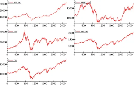
Figure 4.1.1.a Graphs of series at level of stock indices

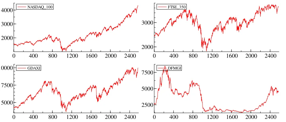
Figure 4.1.1.a and 4.1.1.b given above show in the beginning all series have upward trend than

sharp decline and then again there is an upward trend continuously. This means that series are

Hang Seng (HIS), Standard and Poor (S&P 500) and Dow Jones. In figure 4.1.1.b the series are

Nasdaq 100, FTSE 350, GDAXI, Dubai financial market (DFMGI). Daily data is used from 3rd

Jan, 2005 to 28th Nov, 2014.

Figure 4.1.1.b Graphs of series at level KSE100

0 400 800 1200 1600 2000 2400 10000

20000

30000 KSE100 NIKKI_225

0 400 800 1200 1600 2000 2400 10000

15000

NIKKI_225

HSI

0 400 800 1200 1600 2000 2400 20000

30000 HSI S&P500

0 400 800 1200 1600 2000 2400 1000

1500

2000 S&P500

DJI

0 400 800 1200 1600 2000 2400 10000

15000

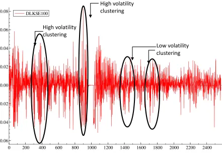
Figure 4.1.2 given below represents return series of Karachi stock market indices. It is

impossible to find out robust model if the series is trendy, we use log difference return series to

deal with trend. In financial econometrics, spread characterized as volatility. In return series spread

does not remain constant, it is known as Hetroscedasticity. The circles in figure 4.1.2 are indicating

the low and high volatility which denote the spread autocorrelation. According to “The Efficient

Market Hypothesis (EMH) return are unpredictable and show mean reversion behavior”. That’s why all

return series have mean reversion behavior. If we combine all effects it indicate ARCH (Auto-Regressive

Conditional Hetroscedasticity) effect. We can easily distinguish between low volatility clustering

and high volatility clustering period. The greater depreciation from constant level (mean of

return series) indicates high volatility clustering and less depreciation illustrate low volatility

clustering. In the same way we can plot and analyze return series of other stock markets.

Figure 4.1.2 Graph of given return series

NASDAQ_100

0 400 800 1200 1600 2000 2400 2000

3000

4000 NASDAQ_100 FTSE_350

0 400 800 1200 1600 2000 2400 2000

3000

FTSE_350

GDAXI

0 400 800 1200 1600 2000 2400 5000

7500

10000 GDAXI DFMGI

0 400 800 1200 1600 2000 2400 2500

5000

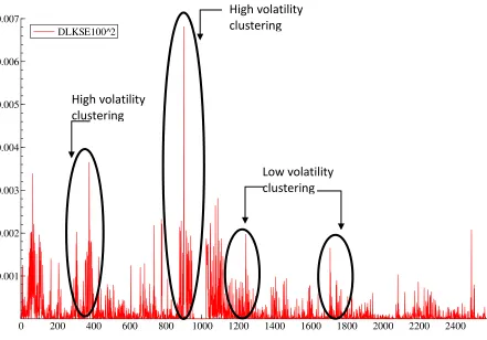
In figure 4.1.3 given below shows squared returns series of KSE 100. The graph of square return

series have “spiky” look signifying variation in square return. Circles indicate high volatility and

low volatility. It also shows that extreme values (outliers) of return series contribute more to the

high volatility. Square of the return series is also known as variance of the return series means

these graphs illustrate the dispersion. In the same way we can analyze square return series of

other stock markets’ indices.

Figure 4.1.3 Graph of Squared return series

DLKSE100

0 200 400 600 800 1000 1200 1400 1600 1800 2000 2200 2400 -0.06

-0.04 -0.02 0.00 0.02 0.04 0.06

0.08 _DLKSE100

High volatility clustering

High volatility clustering

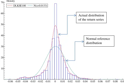
The figure 4.1.4 given below illustrates the distribution of the return series. The distribution of

return series is non-normal. In this graph blue line shows the normal reference distribution of

return series. The red line indicates the actual distribution of the return series. Histograms

describe the outliers (extreme values) in return series. The distribution of return series have

heavy tails and is leptokurtic. This all is due to different response of market players by having

same information from the same market.

Figure 4.1.4 Graphs distribution of the return series

DLKSE100^2

0 200 400 600 800 1000 1200 1400 1600 1800 2000 2200 2400 0.001

0.002 0.003 0.004 0.005 0.006 0.007

DLKSE100^2

High volatility clustering

High volatility clustering

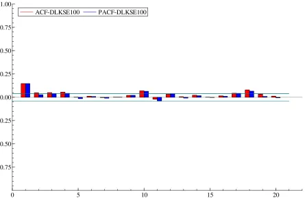
In figure 4.1.5 given below presents ACF (Auto-correlation function) and PACF (Partial

Auto-correlation function) of return series. The green straight lines in this graph show 95 percent

confidence interval, if any bar of ACF and PACF outside these lines means at that lag the values

are auto correlated in other words significantly vary from zero. The ARMA (p, q) process

specify through the significant lags of ACF and PACF. The ACF specify the MA (q) process

PACF specify the AR (p) process. In this graph 1st, 2nd, 3rd, 4th, 10th, 17th and 18th lags of ACF

are significant and 1st, 3rd, 4th, 10th, 11th, 12th, 17th and 18th lags of PACF are significant, these

lags format ARMA (p, q) process in conditional mean equation. It means auto correlation and

partial autocorrelation exist in the return series. We can also analyze cyclical behavior in return

series through ACF and PACF graphs.

Figure 4.1.5 Graphs of ACF and PACF of return series

DLKSE100 N(s=0.0133)

-0.06 -0.05 -0.04 -0.03 -0.02 -0.01 0 0.01 0.02 0.03 0.04 0.05 0.06 0.07 0.08 0.09 10

20 30 40 50 60

70 Density

DLKSE100 N(s=0.0133)

Actual distribution of the return series

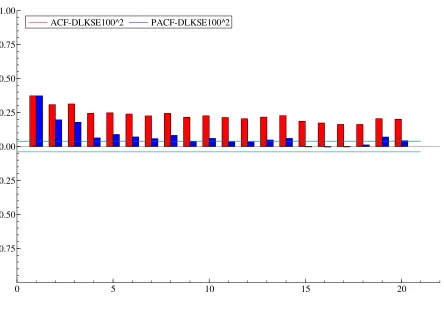
Figure 4.1.6 given below show the graph of ACF and PACF of square return series. 1st to

20th lags of ACF are significantly differ from zero and 1st……...8th, 10th, 13th, 14th, 19th and 20th

lags of PACF are statistically significant. In the same manner square return series ACF and

PACF may provide an indication about the critical lags in conditional variance equation structure

of GARCH (p, q) model. Means there is autocorrelation and partial autocorrelation in the square

return series.

Figure 4.1.6 Graphs of ACF and PACF of square of return series

ACF-DLKSE100 PACF-DLKSE100

0 5 10 15 20

-0.75 -0.50 -0.25 0.00 0.25 0.50 0.75 1.00

The initial statistics of return series of stock markets indices are given below unveil some

indications about the behavior of stock markets. The distributions of return are non-normal,

heavy tails and leptokurtic. The mean of all return series are about zero which implies that return

series show mean reversion behavior. Standard deviation of return series describe the dispersion

from mean value which return series have greater standard deviation it means more deviation

from mean value. The skewness deals with the asymmetry of the distribution. The distributions

of KSE 100, S&P 500, NASDAQ 100, DJI, NIKKEI 225, FTSE 350 and DFMGI return series

are negatively skewed which means that the return of these stock markets are less than average

return. The distributions of HIS and GDAXI are positively skewed which imply the returns of

these markets are more than average return. The Jarque-Bera test with null hypothesis of normal

distribution is employed. Jarque-Bera statistics of all return series are significant means the

distribution of all return series are non-normal.

Table 4.2 Summary statistics

ACF-DLKSE100^2 PACF-DLKSE100^2

0 5 10 15 20

-0.75 -0.50 -0.25 0.00 0.25 0.50 0.75 1.00

Variables

Summary statistics

Mean Standard

deviation

Skewness Jarque

Bera

Excess

Kurtosis

Q-stat (5)

Q2_-stat (5) ARCH 1-2 KPSS KSE 100

0.0006 0.0132 -0.3854 (0.000) 1098.1 (0.000) 3.1075 (0.000) 76.120 (0.000) 1167.51 (0.000) 266.88 (0.000) 0.2073 S&P 500

0.0002 0.0127 -0.3409 (0.000) 14088 (0.000) 11.448 (0.000) 45.484 (0.000) 1131.31 (0.000) 266.72 (0.000) 0.1965 NASDAQ

100 0.0003 0.0136 -0.1587

(0.000) 7985.9 (0.000) 8.6282 (0.000) 24.928 (0.000) 765.777 (0.000) 156.96 (0.000) 0.2005

DJI _{0.0001 0.0116 -0.0851}

(0.077) 14168 (0.000) 11.499 (0.000) 45.037 (0.000) 1123.85 (0.000) 283.89 (0.000) 0.1548 NIKKEI 225

0.0001 0.0153 -0.5737 (0.000) 8597.9 (0.000) 8.8850 (0.000) 10.564 (0.000) 1396.71 (0.000) 489.45 (0.000) 0.1994

HIS _{0.0002 0.0156 0.0459}

(0.000) 10971 (0.000) 10.120 (0.000) 8.3870 (0.000) 1361.38 (0.000) 361.66 (0.000) 0.0525 FTSE 350

0.0001 0.0118 -0.1879 (0.000) 7288.8 (0.000) 8.2401 (0.000) 39.367 (0.000) 1130.0 (0.000) 147.29 (0.000) 0.0569

GDAXI _{0.0003 0.0137 0.0297}

(0.537) 5510.5 (0.000) 7.1719 (0.000) 16.783 (0.000) 686.71 (0.000) 111.39 (0.000) 0.07411

DFMGI _{0.0001 0.0183 -0.8778}

Null Hypotheses (All Null Hypotheses are for nth _order)

KPSS H0: Return series is level stationary, Asymptotic significant values 1% (0.739), 5% (0.463), 10%

(0.347). Q-stat (return series) there is no serial autocorrelation. Q2_{-stat (square return series) H0: there is}

no serial autocorrelation. Jarque-Bera H0: distribution of series is normal. LM-ARCH H0: there is no

ARCH effect. Use these Asymptotic Significance values of t-stat 1% (0.01), 5% (0.05), 10% (0.1) and compare these critical values with P-values (Probability values). P-values are in the parenthesis.

The Excess kurtosis of all returns series are significant which means that return series

distributions are leptokurtic and also indicates that probability of large values is more than

normal return series. Q-stat of return series are significant, rejecting the null hypothesis of no

autocorrelation return series. This shows that there is serial autocorrelation in return series.

Q-stat of squared return series are significant, rejecting the null hypothesis of no autocorrelation in

squared return series. This shows that there is serial autocorrelation in square return series.

LM-ARCH test validates that there is LM-ARCH effect in return series. KPSS is a unit root test with null

hypothesis of stationary series. KPSS test results of all variable show that the estimated values

lies in acceptance region [less than given three significance values 1% (0.739), 5% (0.463), 10%

(0.347)] means the null hypothesis is accepted, return series are level stationary.

4.3 Volatility Model specifications of Return Series

In this section volatility models of stock markets (area under study) are presented to understand

the Data Generating Process of all financial return series (area under study). It will be helpful to

understand the mean and volatility structure of financial return series (area under study).

Volatility modeling is a striking issue for market players, portfolio managers, academicians and

policy makers. A lot of empirical work on volatility modeling exists in financial econometrics,

the predictability and modeling of volatility is still a challenge for researchers. Many researcher

in their studies employed GARCH type model for volatility modeling. In these studies

researchers employed different ARCH-GARCH family models to describe volatility modeling

and volatility forecasting [Vijayalakshmi and Gaur (2013); Pasha et al. (2007); Kamal et al.

(2011); Khan and Parvez (2013); Chand et al. (2013); Jabeen and Saud (2014); Sajid et al. (2012)

and Faisal et al. (2012)]. In this study we employ GARCH (p, q) and GJR (p, q) model for

employed by the researchers due to unique characteristics of these models. These univariate

models are best to give a better explanation of asset volatility modeling.

The GARCH model is employed for HIS volatility modeling. The estimated conditional mean

equation (4.1) is from equation (3.5) and the estimated conditional dispersion equation (4.2) is

from equation (3.6). The P-values are in parenthesis.

𝑅

= 0.0005

……… (4.1)

σ

= 0.0077 + 0.0523ε

2

+ 2.0077σ

t−1

2

+ 1.7204σ

t−2

2

+ 0.6600σ

t−3

2

... (4.2)

The GJR model is employed for KSE 100 volatility modeling. The estimated conditional mean

equation (4.3) is from equation (3.9) and the estimated conditional dispersion equation (4.4) is

from equation (3.10). The P-values are in parenthesis.

𝑅

= 0.0008 + 1.0000𝑅

− 0.9000𝜀

……… (4.3)

σ

= 0.0000 + 0.1460ε

+ 0.3234ε

𝐺

+ 0.8031σ

……...….…… (4.4)

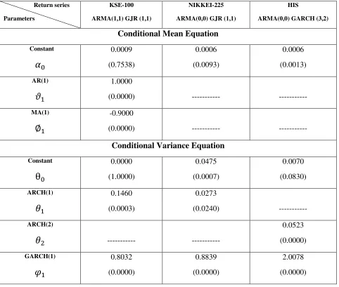
The employed models in table 4.3.1 given below describe the data generating process of the

return series. The estimated parameters of the employed models are statistically significant. In

KSE 100 model AR (1) term is statistically significant which means that current return of KSE

100 depends upon 1st lag. MA (1) term in this model is also differ from zero, shows relationship

between past and current variations. The leverage effect term 𝛿₁ in KSE 100 and NIKKEI 225 models are significant, indicates that the current return negatively correlated with future

volatility, no leverage effect is found in HIS stock return series. Most of the parameters are

statistically significant at 5% level of significance. ARCH and GARCH terms are also significant

the return series are KSE 100, NIKKEI 225 and HSI all are close to 1 which means that the

persistence of ARCH and GARCH effect take long time to decay.

Tables 4.3.1 also illustrate the post estimation results (Residual analysis). The Jarque Bera test

(Normality test) results show non normal residuals. The Q-stat are insignificant up to 10th lags

accept null hypothesis means no serial autocorrelation in the standardized residuals. The Q-stat

on squared standardized residuals are insignificant up to 10th lags accept null hypothesis means

no serial autocorrelation in squared standardized residuals. LM-ARCH test is also insignificant

up to 5th_{lags accept null hypothesis means no ARCH effect remain in series residuals.}

Table 4.3.1 Volatility models of Asian Stock markets Return series

Return series

Parameters

KSE-100

ARMA(1,1) GJR (1,1)

NIKKEI-225

ARMA(0,0) GJR (1,1)

HIS

ARMA(0,0) GARCH (3,2)

Conditional Mean Equation

Constant

𝛼

𝜗

(0.0000) --- ---

MA(1)

∅

-0.9000

(0.0000) --- ---

Conditional Variance Equation

Constant

θ

𝜃

(0.0240) ---

ARCH(2)

𝜃

GARCH(2)

𝜑

1.7205

(0.0000)

GARCH(3)

𝜑

0.6600 (0.0000) GJR(1)

𝛿

(0.0000) ---

Persistence of shock _{1.1109 0.9755 0.9996}

Null Hypotheses(All Null Hypotheses are for nth order)

AR (p) H0: 𝜗_𝑖= 0 No AR Process, MA (q) H0: ∅_𝑖= 0 No MA Process, ARCH H0: 𝜃_𝑖= 0 No ARCH effect, GARCH H0: 𝜑_𝑖= 0 No GARCH effect, Leverage effect H0: 𝛿_𝑖= 0 No leverage effect. P-values are in the parenthesis.

Residual Analysis Parameter Series Jarque Bera Q-Stat (5) Q-Stat (10)

Q2_-Stat

(5)

Q2_-Stat

(10) LM -ARCH (1-2) LM-ARCH (1-5) HIS 128.04 (0.0000) 1.7793 (0.8787) 5.1972 (0.8776) 5.2051 (0.3913) 13.983 (0.5267) 0.3964 (0.6727) 0.5536 (0.7356) NIKKEI 225 509.46 (0.0000) 2.0605 (0.8407) 6.0220 (0.8134) 0.6678 (0.8807) 5.1253 (0.7440) 0.2047 (0.8149) 0.1380 (0.9835) KSE 100 7.0272 (0.0000) 0.0019 (0.9999) 0.0024 (1.0000) 0.0020 (0.9999) 0.0039 (1.0000) 0.0004 (0.9999) 0.0004 (1.0000)

Null Hypotheses(All Null Hypotheses are for nth _order)

Q-stat (return series) there is no serial autocorrelation. Q2_{-stat (square return series) H0: there is no serial}

autocorrelation. Jarque-Bera H0: distribution of series is normal. LM-ARCH H0: there is no ARCH effect.

P-values are in the parenthesis.

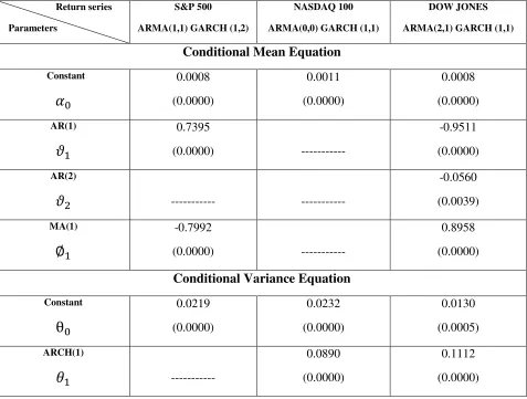
The employed models given below in table 4.3.2 describe the data generating process of

the return series. The estimated parameters of the fitted models are statistically significant. In

S&P 500 and DOW JONES models AR term is statistically significant which means that current

return of these market are only depends upon lag values. In NASDAQ model AR term is

term in S&P 500 and DOW JONES model is differ from zero, shows relationship between past

and current variations of return series. Most of the parameters are statistically significant at 5%

level of significance. ARCH and GARCH terms are also significant in three models means these

return series encompass ARCH and GARCH effect. The persistence of shock of the return series

are S&P 500, NASDAQ 100 and DOW JONES all are close to 1 which means that the

persistence of ARCH and GARCH effect take long time for decay.

Table 4.3.2 also illustrate the post estimation results (Residual analysis). The Jarque Bera test

(Normality test) results show non normal residuals. The Q-stat are insignificant up to 10th _lags

accept null hypothesis means no serial autocorrelation in the standardized residuals. The Q-stat

on squared standardized residuals are insignificant up to 10th _{lags accept null hypothesis means}

no serial autocorrelation in squared standardized residuals.

Table 4.3.2 Volatility models of American Stock markets Return series

Return series

Parameters

S&P 500

ARMA(1,1) GARCH (1,2)

NASDAQ 100

ARMA(0,0) GARCH (1,1)

DOW JONES

ARMA(2,1) GARCH (1,1)

Conditional Mean Equation

Constant

𝛼

𝜗

(0.0000) ---

-0.9511

(0.0000)

AR(2)

𝜗

-0.0560

(0.0039)

MA(1)

∅

-0.7992

(0.0000) ---

0.8958

(0.0000)

Conditional Variance Equation

Constant

θ

𝜃

0.0890

(0.0000)

0.1112

ARCH(2)

𝜃

0.1433

(0.0000) --- ---

GARCH(1)

𝜑

Persistence of shock _{0.9915 0.9883 0.9954}

Null Hypotheses(All Null Hypotheses are for nth order)

AR (p) H0: 𝜗_𝑖= 0 No AR Process, MA (q) H0: ∅_𝑖= 0 No MA Process, ARCH H0: 𝜃_𝑖= 0 No ARCH effect, GARCH H0: 𝜑_𝑖= 0 No GARCH effect. P-values are in the parenthesis.

Residual Diagnostic Test

Parameter Series Jarque Bera Q-Stat (5) Q-Stat (10)

Q2_-Stat

(5)

Q2_-Stat

(10) LM -ARCH (1-2) LM-ARCH (1-5) S&P 500 524.96 (0.0000) 4.5842 (0.2049) 7.4715 (0.4867) 1.2465 (0.5361) 9.7895 (0.2008) 0.2319 (0.7930) 0.2597 (0.9350) NASDAQ 100 213.74 (0.0000) 2.8643 (0.2387) 5.1957 (0.6360) 5.8315 (0.1201) 14.408 (0.0717) 2.7272 (0.0656) 1.1573 (0.3279) DJI 438.61 (0.0000) 5.2781 (0.0714) 8.9697 (0.2548) 8.5410 (0.0360)* 17.475 (0.0255)* 3.8500 (0.0214)* 1.6483 (0.1438)

Null Hypotheses(All Null Hypotheses are for nth _order)

Q-stat (return series) there is no serial autocorrelation. Q2_{-stat (square return series) H0: there is no serial}

autocorrelation. Jarque-Bera H0: distribution of series is normal. LM-ARCH H0: there is no ARCH effect.

P-values are in the parenthesis.

LM-ARCH test is also insignificant up to 5thlags accept null hypothesis means no ARCH effect

remain in series residuals.

In table 4.3.3 given above describes the data generating process of the return series. The

estimated parameters of the fitted models are statistically significant. In GDAXI and DFMGI

models AR terms are statistically significant which means that current return of markets are only

this market not depends upon lag values. MA (1) term in GADXI and DFMGI models are differ

from zero, shows relationship between past and current variations of return series. Most of the

parameters are statistically significant at 5% level of significance. ARCH and GARCH terms are

also significant in three models means these return series encompass ARCH and GARCH effect.

The persistence of shock of the return series are FTSE 350 (0.99359), GDAXI (0.99321) and

DFMGI (0.99417) all are close to 1 which means that the persistence of ARCH and GARCH

effect take long time for decay.

Table 4.3.3 also illustrate the post estimation results (Residual analysis). The Jarque Bera test

(Normality test) results show non normal residuals. The Q-stat are insignificant up to 10th lags

accept null hypothesis means no serial autocorrelation in the standardized residuals. The Q-stat

on squared standardized residuals are insignificant up to 10th lags accept null hypothesis means

no serial autocorrelation in squared standardized residuals. LM-ARCH test is also insignificant

up to 5thlags accept null hypothesis means no ARCH effect remain in series residuals.

Table 4.3.3 Volatility models of European and Gulf Stock markets Return series

Return series

Parameters

FTSE 350

ARMA(0,0) GARCH (1,1)

GDAXI

ARMA(1,1) GARCH (1,1)

DFMGI

ARMA(1,1) GARCH (1,1)

Conditional Mean Equation

Constant

𝛼

𝜗

0.9396

(0.0000)

0.8848

(0.0000)

MA(1)

∅

-0.9551

(0.0000)

-0.8330

(0.0000)

Conditional Variance Equation

GARCH(1)

𝜑

Persistence of shock _{0.9935 0.9932 0.9941}

Null Hypotheses(All Null Hypotheses are for nth order)

AR (p) H0: 𝜗_𝑖= 0 No AR Process, MA (q) H0: ∅_𝑖= 0 No MA Process, ARCH H0: 𝜃_𝑖= 0 No ARCH effect, GARCH H0: 𝜑_𝑖= 0 No GARCH effect, Mean spillover. P-values are in the parenthesis.

Residual Analysis Parameter Series Jarque Bera Q-Stat (5) Q-Stat (10)

Q2_-Stat

(5)

Q2_-Stat

(10) LM -ARCH (1-2) LM-ARCH (1-5) FTSE 350 134.01 (0.0000) 3.5698 (0.6128) 5.2425 (0.8743) 3.7790 (0.2863) 5.0251 (0.7548) 0.6032 (0.5471) 0.7742 (0.5682) GDAXI 309.27 (0.0000) 4.5445 (0.2083) 7.4357 (0.4904) 6.9227 (0.0744) 8.9998 (0.3423) 0.8606 (0.4230) 1.4246 (0.2121) DFMGI 12835 (0.0000) 6.7335 (0.0808) 12.502 (0.1301) 3.4343 (0.3293) 8.3277 (0.4021) 0.2255 (0.7981) 0.6888 (0.6319)

Null Hypotheses(All Null Hypotheses are for nth _order)

Q-stat (return series) there is no serial autocorrelation. Q2_{-stat (square return series) H0: there is no serial}

autocorrelation. Jarque-Bera H0: distribution of series is normal. LM-ARCH H0: there is no ARCH effect.

P-values are in the parenthesis.

Conclusion

This study has offered a framework to model the time varying volatility of equity markets by

employing the risk models. On the basis of given data sets we employed symmetric GARCH

and asymmetric GARCH models to estimate conditional mean equations follow ARMA process

and conditional variance equations for risk (dispersion). For the validity of models the residual

diagnostic test also employed. KSE 100 and NIKKEI 225 series have asymmetric effect while

persistence of ARCH and GARCH effect in return series. The leverage effects are also quantified

to check the effects of different news on volatility.

REFERENCES

Attari, M. I. J., Safdar, L., & Student, M. B. A. (2013). The Relationship between Macroeconomic

Volatility and the Stock Market Volatility: Empirical Evidence from Pakistan. Pakistan Journal of

Commerce and Social Sciences, 7(2), 309-320.

Abou-Zaid, A. S. (2011). Volatility spillover effects in emerging MENA stock markets. Review of

Applied Economics, 7(1-2).

Ali, R., & Afzal, M. (2012). Impact of global financial crisis on stock markets: Evidence from Pakistan

and India. E3 Journal of Business Management and Economics, 3(7), 275-282.

Black, F. (1976). Stuedies of stock price volatility changes. Journal of American Statistical Association,

177-181.

Bollerslev, T. (1986). Generalized autoregressive conditional heteroskedasticity. Journal of econometrics,

31(3), 307-327.

Bashir, R., Shakir, R., Ashfaq, B., & Hassan, A. (2014). The Efficiency of Foreign Exchange Markets in

Pakistan: An Empirical Analysis. The Lahore Journal of Economics, 19(1), 133.

Bollerslev, T., & Mikkelsen, H. O. (1996). Modeling and pricing long memory in stock market volatility.

Bollerslev, T., Litvinova, J., & Tauchen, G. (2006). Leverage and volatility feedback effects in

high-frequency data. Journal of Financial Econometrics, 4(3), 353-384.

Choi, D. F., Fang, V., & Fu, T. Y. (2010). Volatility spillovers between New Zealand stock market

returns and exchange rate changes before and after the 1997 Asian financial crisis. Asian Journal of

Finance & Accounting, 1(2).

Engle, R. F. (1982). Autoregressive conditional heteroscedasticity with estimates of the variance of

United Kingdom inflation. Econometrica: Journal of the Econometric Society, 987-1007.

Engle, R. F., & Ng, V. K. (1993). Measuring and testing the impact of news on volatility. The journal of

finance, 48(5), 1749-1778.

Engle, R. F., Ito, T., & Lin, W. L. (1990). Meteor Showers or Heat Waves? Heteroskedastic Intra-Daily

Volatility in the Foreign Exchange Market." Econometrica 58 (3).

Glosten, L. R., Jagannathan, R., & Runkle, D. E. (1993). On the relation between the expected value and

the volatility of the nominal excess return on stocks. The journal of finance, 48(5), 1779-1801.

Granger, C. W. J., & Andersen, A. (1978). On the invertibility of time series models. Stochastic processes

and their applications, 8(1), 87-92.

Gomez, S., & Ahmad, H. (2014). Volatility transmission between PALS, FOES, MINIONS and TITANS.

Jabeen, M., & Khan, S. A. (2014). Modelling Exchange Rate Volatility by Macroeconomic Fundamentals

in Pakistan. International Econometric Review (IER), 6(2), 58-76.

Khalil, M. Z., Usman, M., & Shafique, I. (2013). Volatility Spill-over between the Stock Market and the

Foreign Exchange Market in Pakistan. Management and Administrative Sciences Review, 2(6), 695-704.

Mushtaq, R., Zia ur Rehman, M., Ali Shah, S. Z., & Murtaza, G. (2011). Sources of Return and Volatility

Spillover for Pakistan: An Analysis of Exogenous Factors by using EGARCH Model. International

Conference on Business and Economics Research, 16, 151-157.

Padhi, P., & Lagesh, M. A. (2012). Volatility Spillover and Time-Varying Correlation among the Indian,

Asian and US Stock Markets. Journal of Quantitative Economics, 10(2), 78-90.

Qayyum, A., & Kemal, A. R. (2006). Volatility spillover between the stock market and the foreign

exchange market in Pakistan. PIDE Working Paper 2006:7.

Qayyum, A., & Khan, M. A. (2014). Dynamic Relationship and Volatility Spillover between the Stock

Market and the Foreign Exchange Market in Pakistan: Evidence from VAR-EGARCH Modelling. PIDE

Working Papers 103.

Sok-Gee, C., Karim, M. A., & Karim, M. A. (2010). Volatility spillovers of the major stock markets in

ASEAN-5 with the US and Japanese stock markets. International Research Journal of Finance and

Economics, 44, 161-72.

Sinha, P., & Sinha, G. (2010). Volatility Spillover in India, USA and Japan Investigation of Recession

Tahir, S. H., Sabir, H. M., Ali, Y., Ali, S. J., & Ismail, A. (2013). Interdependence of South Asian &

Developed Stock Markets and Their Impact on KSE (Pakistan). Asian Economic and Financial Review,

3(1), 16-27.

Yang, S. Y., & Doong, S. C. (2004). Price and volatility spillovers between stock prices and exchange

rates: empirical evidence from the G-7 countries. International Journal of Business and Economics, 3(2),

139.

Zia, Q. Z., & Rahman, Z. (2011). The causality between stock market and foreign exchange market of