Munich Personal RePEc Archive
How much can we identify from repeated
games?
Abito, Jose Miguel
University of Pennsylvania
31 August 2015
Online at
https://mpra.ub.uni-muenchen.de/66378/
How much can we identify from repeated games?
Jose Miguel Abito∗
August 31, 2015
[PRELIMINARY DRAFT. COMMENTS ARE WELCOME]
Abstract
I propose a strategy to identify structural parameters in infinitely repeated games without
relying on equilibrium selection assumptions. Although Folk theorems tell us that almost any
individually rational payoff can be an equilibrium payoff for sufficiently patient players, Folk
theorems also provide tools to explicitly characterize this set of payoffs. I exploit the extreme
points of this set to bound unobserved equilibrium continuation payoffs and then use these to
generate informative bounds on structural parameters. I illustrate the identification strategy
using (1) an infinitely repeated Prisoner’s dilemma to get bounds on a utility parameter, and
(2) an infinitely repeated quantity-setting game to get bounds on marginal cost and provide a
robust test of firm conduct.
1
Introduction
The application of game theoretical models and insights to empirical settings has been critical
in capturing strategic interaction among economic agents in empirical work.1 By combining
as-sumptions on agents’ rationality and an equilibrium concept, empirical researchers are able to link
observed behavior with underlying model primitives such as agents preferences and constraints.
Rationality allows one to put structure on how primitives translate to individual incentives for
a given action. Because of strategic interaction, an equilibrium concept is used to link different
agents’ individual incentives and beliefs into outcomes in a consistent way.
Multiple equilibria typically precludes a unique mapping from primitives to observed behavior,
making standard inference problematic without additional, often strong, assumptions. An
impor-tant part of the lirerature on the econometrics of games have focused on the multiple equilibria
problem. Substantial progress has been made in the analysis of static games (Tamer (2003),
Cilib-erto and Tamer (2009), Beresteanu, Molchanov, and Molinari (2011), Galichon and Henry (2011)).
However, not much progress has been made for dynamic games. One important class of dynamic
games where identification results are virtually unexplored are repeated games.
Repeated games provide a useful framework to model long-run relationships which lead to
incentives and outcomes that are not otherwise captured by one-shot interactions. The framework
provides insights on how agents can manage to cooperate in a non-cooperative environment without
formal or explicit contracts, and how to build a reputation. Despite the richness of repeated games,
there is some apprehension in its use due to the framework’s general inability to make sharp
predictions (Dal B´o and Fr`echette, 2011). This has hampered the use of repeated games both in
applied theory and empirical research. The multiplicity problem in repeated games is so perverse
that a significant part of the theoretical literature has been devoted to deriving Folk Theorems
that basically say that almost any individually rational payoff can be sustained as an equilibrium
payoff. Thus, an open question in applying repeated games to empirical work is whether we can
even learn anything from the data despite the Folk Theorem.
I develop an empirical strategy to identify structural parameters of infinitely repeated games
without equilibrium selection assumptions. This strategy allows one to determine how much we
can learn from the data just from the game’s basic structure. Moreover, it provides a strategy that
that can be used in empirical research involving repeated games.
The identification problem and the consequent strategy is as follows. Actions taken by players
today depend on what players expect to happen in the future. The one-stage deviation principle
(OSDP) allows us to rationalize a given player’s chosen action (conditional on the rival’s) as an
inequality comparing the sum of stage game payoffs and equilibrium continuation payoffs for the
chosen action versus the best single-stage deviation. While OSDP simplifies the analysis by limiting
to equilibrium continuation payoffs, analysis remains complicated since (almost) any individually
rational payoff can be sustained as an equilibrium continuation payoff as long agents are sufficiently
patient. Hence, there are potentially infinitely many ways to rationalize observed actions and so one
cannot directly invert the mapping from observed actions to primitives unless we know or assume
what equilibrium is being played.
Folk Theorems explictly characterize the set of equilibrium (average) continuation payoffs. I
show how to use extreme points of this set to generate informative bounds on the structural
pa-rameter given data on frequency of stage game action profiles. While inference is limited to sets
instead of singleton estimates of primitives (partial identification), the proposed identification
strat-egy reveals that the basic structure of repeated games is quite informative about agents’ primitives
despite the Folk Theorem. Moreover, I show that set estimates of primitives can be used to provide
a useful test of behavior (firm conduct).
In section 2, I start off with an analysis of a standard infinitely-repeated Prisoner’s Dilemma
to illustrate the identification strategy in a simple and familiar setting. I show how bounds on a
utility parameter can be constructed using the incentive constraints from OSDP, and the upper
and lower bounds of the set of equilibrium average payoffs from the Folk Theorem. Moreover, I
model.
The analysis of the Prisoner’s Dilemma yields general insights on identification. First, there
are two levels of equilibrium selection assumptions–a static equilibrium selection assumption and a
dynamic one. Dynamic equilibrium selection assumptions refer to assumptions on how players will
play the game in the future which maps to what equilibrium continuation payoffs are. However,
de-spite knowing what equilibrium continuation payoffs are, the model still turns out to beincomplete,
in the sense similar to the multiple equilibrium problem in static games (Tamer, 2003). Finally,
even if both static and dynamic equilibrium selection assumptions are made, point identification
may still fail if there is no ample source of variation that the econometrician has some knowledge
of (i.e. either this variation is observed or has some known distribution).
In section 3, I discuss the identification strategy in a more general setting. The same key
ideas of using OSDP and the Folk Theorem drives the identification strategy. I then apply the
identification strategy to a quantity-setting game in section 4. This application differs from the
Prisoner’s Dilemma in an important way. In the Prisoner’s Dilemma, the econometrician explicitly
observes stage game actions “Cooperate” or “Deviate” which contains some information on players’
long-run strategies. In the quantity-setting game, I assume that the econometrician only observes
the actual values of the quantities chosen, and not whether these quantities map to “Cooperate”
(e.g. joint monopoly quantity) or “Deviate” (e.g. Cournot quantity). I derive bounds for marginal
cost and show how parameters of the model affect informativeness of these bounds. Finally I show
how one can use the set estimates of marginal cost to test for firm conduct.
The identification strategy can be adapted to other dynamic games, specifically to stochastic
games. Stochastic games with Markovian strategies are widely used in fields such as industrial
organization and labor, although actual estimation of these games has been more limited. Moreover,
feasibility of current methods require an equilibrium selection assumption. The advantage of my
identification strategy is that it does not require equilibrium selection assumptions. Although the
strategy requires knowing something about equilibrium continuation payoffs, there is no need to
be easier to compute. I offer more discussion at the end in section 5.
2
Example: Prisoner’s Dilemma
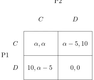
Figure 1 is a Prisoner’s dilemma with unknown utility parameter α ∈ (0,5). The goal of the
econometrician is to estimate α given data on outcomes. Suppose this game is repeated infinitely
many times with discount factorδ. Assume that the econometrician observes a sample of actions, i.e.
stage game outcomes, and also the discount factor. For now let us assume that the econometrician
observes a time series of stage game outcomes for a single market (or prison).
P1
P2
C D
C α, α α−5,10
[image:6.612.228.385.319.452.2]D 10, α−5 0,0
Figure 1: Prisoner’s dilemma stage game payoffs
To estimateα, we want to link observed frequencies of stage outcomes with predicted frequencies
coming from a theoretical model. Consider observing the frequency of (C, C) in the data, i.e.
Pr(C, C). The one-stage deviation principle (OSDP) allows us to characterize a player’s incentive
to choose C when the rival choosesC as an inequality
(1−δ)α+δvCC|h≥(1−δ)10 +δvCD|h
where vkk′|h’s are equilibrium average continuation payoffs proceeding immediately the outcome
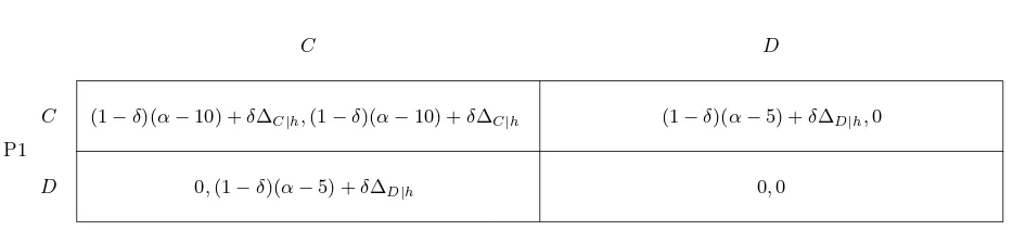
(k, k′) and history h. Let ∆C|h≡vCC|h−vDC|h and ∆D|h≡vDD|h−vDC|h. Using the OSDP, the
normal form game in figure 2 for a given history h. This gives necessary and sufficient conditions
on when we will observe the stage game outcome (C, C and hence the frequency of this outcome
occuring.
P1
P2
C D
C (1−δ)(α−10) +δ∆C|h,(1−δ)(α−10) +δ∆C|h (1−δ)(α−5) +δ∆D|h,0
[image:7.612.74.541.207.313.2]D 0,(1−δ)(α−5) +δ∆D|h 0,0
Figure 2: Normal form game using one-stage deviation principle: Prisoner’s Dilemma
A necessary condition for observing (C, C) given history h is that it is a Nash equilibrium of
the normal form game. If we restrict to pure strategies, this necessary condition is given by2
(1−δ)(α−10) +δ∆C|h >0.
Thus,
Pr(C, C|h)≤Pr((1−δ)(α−10) +δ∆C|h>0|h). (1)
Similarly, a sufficient condition for observing (C, C) given history h is that it is the unique Nash
equilibrium of the normal form game:
(1−δ)(α−10) +δ∆C|h >0∩(1−δ)(α−5) +δ∆D|h>0
and so
Pr((1−δ)(α−10) +δ∆C|h >0∩(1−δ)(α−5) +δ∆D|h>0|h)≤Pr(C, C|h). (2)
2If we allow for (uncorrelated) mixed strategies, then there is a mixed strategy equilibrium involving each player
choosingCwith probabilityρ= (1−δ)(α−5)+δ∆D|h
(1−δ)5+δ(∆D|h−∆C|h). In order forρ∈(0,1), we need (1−δ)(α−10) +δ∆C|h<0 and
(1−δ)(α−5) +δ∆D|h>0. Thus, Pr(C, C|h)≤Pr((1−δ)(α−10) +δ∆C|h>0|h) +ρ·Pr[(1−δ)(α−10) +δ∆C|h<
The above analysis shows that despite knowing the equilibrium continuation payoffs (∆C|h,∆D|h),
the model is still incomplete in that we cannot write the likelihood for (C, C) (given h) (Tamer,
2003). In this sense, we have a static equilibrium selection problem on top of the dynamic
equi-librium selection problem, i.e. knowing the equiequi-librium continuation payoffs. The identification
strategy deals with both the static and dynamic equilibrium selection problems.
2.1 Deriving the identified set
LetF∆h as the joint distribution of (∆C|h,∆D|h). This distribution captures the dynamic
equilib-rium selection mechanism. Dynamic equilibequilib-rium selection assumptions are essentially assumptions
onF∆h. For example, if we assume that players are implementing a Grim-Trigger strategy that
sus-tains (C, C) forever using a punishment of (D, D), thenF∆h puts all its mass on ∆C|h =α−0 =α
and ∆D|h = 0−0 = 0 for histories involving cooperation in the past, and ∆C|h = ∆D|h = 0 for
histories where some deviation in the past occurred.
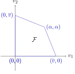
v1
v2
(0,0) (v,0) (0,0)
(0, v)
(α, α)
[image:8.612.234.380.405.549.2]F
Figure 3: Set of individually rational payoffs in in our Prisoner’s Dilemma (α∈(0,5))
The Folk Theorem in fact characterizes the set of equilibrium average payoffs for sufficiently
patient players. Specifically, almost any individually rational stage payoff can be sustained as a
of individually rational payoffs for our Prisoner’s Dilemma. Let v(α) and v(α) be the lower and
upper bounds of this set, which are functions of the unknown parameterα. For any discount factor
less than or equal to one, the support of F∆h for any history h must be a subset
3 of the set of
differences in equilibrium payoffs inF, i.e. supp(F∆h)⊆
∆(α),∆(α)
, where ∆(α) =v(α)−v(α)
and ∆(α) =v(α)−v(α). The following proposition shows how one can use thee bounds to derive
an identified set for the unknown parameterα without any equilibrium selection assumptions.
Proposition 1. Assume players are restricted to pure strategies. Moreover, suppose we only
observe the frequency Pr(C, C) and the discount factorδ. The identified set for α is given by
H(α) ={α: Pr(C, C)∈[Pr(LB(α)>0),Pr(U B(α)>0)]}
whereLB(α) = (1−δ)(α−10) +δ∆(α),U B(α) = (1−δ)(α−10) +δ∆(α), ∆(α) = 50−(α−5)(5 α−10)
and ∆(α) =−∆(α).
Proof. Since ∆C|h ≤∆(α) for all histories h, the necessary condition given by inequality 1 implies
Pr(C, C|h)≤Pr((1−δ)(α−10) +δ∆(α)>0).
Integrating this inequality across histories yields
Pr(C, C)≤U B(α)
whereU B(α) = (1−δ)(α−10) +δ∆(α).
Next, since ∆C|h ≥∆(α) and ∆D|h ≥∆(α) for all histories h, the sufficient condition given by
inequality 2 implies
Pr((1−δ)(α−10) +δ∆(α)>0∩(1−δ)(α−5) +δ∆(α)>0)≤Pr(C, C|h).
Integrating this across histories gives
Pr((1−δ)(α−10) +δ∆(α)>0∩(1−δ)(α−5) +δ∆(α)>0)≤Pr(C, C).
3Moreover, since we restrict to pure strategies, the actual set of equilibrium average payoffs is actually a proper
Since (1−δ)(α−10) +δ∆(α) > 0 implies (1−δ)(α−5) +δ∆(α) > 0, the lefthand side of the
above inequality is just equal to
Pr((1−δ)(α−10) +δ∆(α)>0).
Thus,
LB(α)≤Pr(C, C)
whereLB(α) = (1−δ)(α−10) +δ∆(α).
To derive ∆(α) and ∆(α), recall that ∆(α) = v(α)−v(α) and ∆(α)−∆(α). From figure 3,
we have v(α) = 0 while v(α) is characterized by the point (0, v(α)) that lies on the line segment
connecting (α−5,10) and (α, α). (or equivalently, the point (v(α),0) that lies on the line segment
connecting (α, α) and (10, α−5)). After some algebra, one can show thatv(α) = 50−(α−5)(5 α−10).
To explicitly derive the identified set for α, we need to derive all values of α such that the
observed frequency Pr(C, C) is inside the interval [Pr(LB(α),Pr(U B(α))]. Since bothLB(α) and
U B(α) are deterministic functions of α, Pr(LB(α)) = I{LB(α)} and Pr(U B(α)) = I{U B(α)}
whereI{·}is the indicator function. Moreover, sinceLB(α) andU B(α) are continuous functions of
α, the set ofα’s that satisfy Pr(C, C)∈[I{LB(α)},I{U B(α)}] are just a finite union of intervals
over the set of possibleα’s.
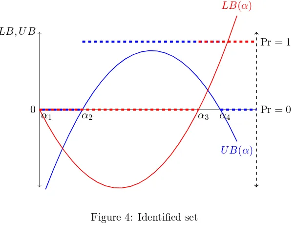
There are three possible identified sets depending on Pr(C, C). Figure 4 illustrates these
iden-tified sets graphically. If Pr(C, C) = 0, then it must be that LB(α) ≤0 which gives some bound
on α, i.e. α ∈ [α1, α3] in figure 4. Notice that there is no restriction provided by U B(α) since
I{U B(α)} can be zero or one. Intuitively, Pr(C, C) = 0 requires that (C, C) is not a unique Nash
equilibrium of the induced normal form game in figure 2. However, Pr(C, C) = 0 does not rule out
that (C, C) can be one of multiple Nash equilibria.
Similarly, if Pr(C, C) = 1, then it must be that U B(α)>0 but there is no restriction provided
byLB(α). Finally, when Pr(C, C)∈(0,1), it must be thatU B(α)>0and LB(α)≤0 since (C, C)
than the other two cases since it provides more restrictions on α. However, different values for
Pr(C, C)∈(0,1) yields the same identified set so what only matters is that the frequency is neither
zero or one, and no additional information is provided. The reason is the following. Variation in
outcomes, say of (C, C), are driven by the distributionF∆h. The shape of this distribution provides
useful information about how outcomes would vary in the sample. However, at this point, we only
know the support of this distribution, specifically, its endpoints, which is not enough to explain what
determines the “non-degenerate” variation leading to specific values for Pr(C, C) ∈ (0,1). Thus
the researcher needs additional known sources of variation, either through an observed variable or
an unobserved variable with some known distribution that moves around payoffs and outcomes.
0 Pr = 0
LB, U B
Pr = 1
U B(α) LB(α)
[image:11.612.158.461.320.550.2]α1 α2 α3 α4
Figure 4: Identified set
Note: Blue and red curves are graphs of U B(α) and LB(α) as defined in Propostion 1, respectively. The dotted
blue and red curves give Pr(U B(α)>0) and Pr(LB(α)>0), respectively. Consider frequency of observing (C, C).
If Pr(C, C) = 0, then H(α) = [α1, α3]. If Pr(C, C) = 1, then H(α) = (α2, α4). Finally, if Pr(C, C) ∈ (0,1), then
2.2 Point identification
As it turns out, knowing how equilibrium is selected (both dynamic and static equilibrium selection)
is not sufficient to get point identification of α. To show this, suppose players are playing
Grim-Trigger strategies and that δ is fixed at some value greater than 0.6, say δ = 0.7 (known to the
researcher). Then the researcher observes Pr(C, C) = 1 and that (1−δ)(α−10) +δα > 0 and
(1−δ)(α−5)<0. These implyα >10(1−δ) = 3 and α <5, which only yields α∈(3,5).
The above example illustrates that knowledge of equilibrium selection is not sufficient to pin
down the value ofα. Additional sources of variation that moves payoffs (and outcomes) are needed
to get point identification. For example, suppose we observe different independent prisons indexed
bym, where all players are playing Grim-Trigger strategies. Suppose the discount factor of prisoners
differ across prisons, say δm, and that we have enough variation in δm. Specifically, we observe
that for prisons with δm > 0.6, Pr(C, C) = 1 while for δm < 0.6, Pr(C, C) = 0. Then we have
(1−δ)(α−10) +δα= 0 for δ = 0.6 which impliesα= 4.
3
Identification strategy
The identification strategy consists of two key ideas. First, we can use the one-stage deviation
principle (OSDP) to derive a set of incentive (inequality) constraints that describe conditions
such that a given outcome is part of an equilibrium. The incentive constraints are functions
of stage game and equilibrium continuation payoffs, and if both are known up to the unknown
parameter, then one can use these constraints to identify the parameter (although we might still
only achieve partial identification due to the static equilibrium selection problem). However, the
econometrician does not typically know what equilibrium strategies are being played hence what
equilibrium continuation payoffs go into these incentive constraints. In fact, there are potentially
infinitely many equilibrium payoffs that are consistent with observed outcomes–a result from Folk
Theorems. The second idea is that we can harness the power of Folk Theorems to provide lower
are monotonic in these payoffs, we can then use the conditions implied by these worse case bounds
to derive an identified set for the unknown parameter.
3.1 Set-up
There are two players choosing actions simultaneously in each period indefinitely with common
discount factorδ. Stage game actions for each playeriare elements of the compact setAi. At this
point, it is not necessary to specify whether actions are discrete or continuous. Moreover, actions
need not have specific meaning as in the Prisoner’s Dilemma, and can just be any real number.
Player i’s payoff is denoted by πi(xi, xj;α) where xi is the chosen action of player i, xj s the
chosen action ofi’s rivalj, and α is some parameter. I assume that the econometrician knows the
functional form ofπi(xi, xj;α) but does not knowα. Additionally, the econometrician observes the
chosen stage game actions{xˆi,xˆj}, and also the frequency that these occur, i.e. Pr(ˆxi,xˆj). Finally,
letx∗i(xj) be thestage gamebest response ofitoj’s actionxj, i.e. x∗i(xj) = arg maxx∈Aiπi(x, xj;α).
This best response can be a function ofα, as long as it can be explictly written.
3.2 One-stage deviation principle (OSDP)
OSDP allows us to focus on single-stage deviations to fully characterize incentives of players for
choosing specific actions. That is, player ichooses ˆxi given j plays ˆxj if and only if
(1−δ)πi(ˆxi,xˆj;α) +δˆvi≥(1−δ)πi(x∗i(ˆxj),xˆj;α) +δv˜i
for some ˆvi,v˜i ∈ V whereV is the set ofequilibriumaverage payoffs. When constructing a deviation
(righthandside of the above inequality), we allow i to deviate only for one period by choosing its
best responsex∗i(ˆxj) but requireito go back to equilibrium play afterwards. Equilibrium play then
leads to player ireceiving equilibrium continuation payoffs (written as an average).
The subgame perfect Nash equilibrium (SPNE) of the infinitely repeated game is a Nash
equi-librium of every possible history. For each (relevant) history, we can define a normal form game
of average discounted payoffs such that observed stage game outcomes are Nash Equilibria of these
normal form games.
The next step is to translate the incentive constraints as bounds on the probability of observing
a given stage outcome. Take for example the stage game outcome (ˆxi,xˆj) chosen under history h.
For this stage game outcome to be a Nash equilibrium in pure strategies of the induced normal
form game, it must be that
(1−δ)πi(ˆxi,xˆj;α) +δvˆi|h≥(1−δ)πi(x∗i(ˆxj),xˆj;α) +δv˜i|h
and
(1−δ)πj(ˆxj,xˆi;α) +δvˆj|h ≥(1−δ)πj(x∗j(ˆxi),xˆi;α) +δv˜j|h
With mixed strategies, the set of conditions will be more complicated though are still functions
of equilibrium average payoffs. We can define these necessary conditions as a set Ψ(ˆxi,xˆj,∆h;α)
such that Ψ(ˆxi,xˆj,∆h;α) is increasing4 in ∆h where ∆h is an appropriately defined difference of
equilibrium average payoffs. Thus for each h, Ψ(ˆxi,xˆj,∆h;α) ⊆ Ψ(ˆxi,xˆj,∆);α), where ∆ is an
upperbound that does not depend on h.
Next, we can derive a set of conditions such that (ˆxi,xˆj) is the unique Nash equilibrium of
the induced normal form game.5. Denote the set of sufficient conditions as Ξ(ˆxi,xˆj,∆h;α) for
each historyh, where again Ξ(ˆxi,xˆj,∆h;α) is increasing in ∆h. Thus for eachh, Ξ(ˆxi,xˆj,∆;α)⊆
Ξ(ˆxi,xˆj,∆h);α), where ∆ is a lowerbound that does not depend on h.
3.3 Main theorem
The following theorem characterizes the identified set for the unknown parameterα.
Theorem 1. Construct Ψ(ˆxi,xˆj,∆h;α) and Ξ(ˆxi,xˆj,∆h;α) such that both are increasing in ∆h.
4That is, Ψ(ˆx
i,xˆj,∆h;α)⊆Ψ(ˆxi,xˆj,∆′h;α) for ∆′h>∆h.
The identified set for α is given by
H(α) = \
(ˆxi,xˆj)
α: Pr(ˆxi,xˆj)∈
Pr(Ξ(ˆxi,xˆj,∆;α),Pr(Ψ(ˆxi,xˆj,∆);α)
Proof. Consider some arbitrary outcome (ˆxi,xˆj,). Since Ψ(ˆxi,xˆj,∆h;α) is necessary for one to
observe (ˆxi,xˆj,) under some historyh in an equilibrium, we have
Pr(ˆxi,xˆj|h)≤Pr(Ψ(ˆxi,xˆj,∆h;α)|h).
Because Ψ(ˆxi,xˆj,∆h;α)⊆Ψ(ˆxi,xˆj,∆;α), we have
Pr(ˆxi,xˆj|h)≤Ψ(ˆxi,xˆj,∆;α)
for all histories. Thus,
Pr(ˆxi,xˆj)≤Ψ(ˆxi,xˆj,∆;α).
Next, a sufficient condition for observing (ˆxi,xˆj,) under some history h in an equilibrium is
captured by the set Ξ(ˆxi,xˆj,∆h);α). Hence,
Pr(Ξ(ˆxi,xˆj,∆h);α)|h)≤Pr(ˆxi,xˆj,|h).
Since Ξ(ˆxi,xˆj,∆h);α) is increasing in ∆h, and after integrating across histories, we have
Pr(Ξ(ˆxi,xˆj,∆);α))≤Pr(ˆxi,xˆj).
Thus for each outcome (ˆxi,xˆj) we can derive an identified set as the set of α’s that satisfy
Pr(ˆxi,xˆj)∈
Pr(Ξ(ˆxi,xˆj,∆;α),Pr(Ψ(ˆxi,xˆj,∆);α)
. The identified set that uses all data, H(α) is
just the intersection of these sets.
An important part of the identification strategy is to construct the set of necessary and sufficient
conditions Ψ(ˆxi,xˆj,∆h;α) and Ξ(ˆxi,xˆj,∆h;α) such that both are increasing in ∆h. For each data
point (ˆxi,xˆj,), we can construct bounds on the probability of observing this data point using the
necessary and sufficient conditions evaluated at the extreme points ∆ and ∆. These lower and
upper envelopes can then be used to identify upper and lower bounds for the unknown parameter.
α
EF∆g(s;α)
Pr(ˆxi,xjˆ )
α∗
U B(α)
LB(α)
[image:16.612.149.465.130.273.2]α α
Figure 5: Graphical illustration of how to derive the identified set
4
Application: Quantity-setting game
I apply the identification strategy to a simple quantity-setting game. There are two firms, firms
1 and 2, competing by choosing how much to produce in each period. The firms compete for an
indefinite amount of periods with a common discount factor δ. For ease of exposition, I restrict
quantities to two levels: low quantityqL or high quantity qH, whereqL< qH.6 I assume firms are
symmetric and have a constant marginal cost ofc. Finally, inverse demand is given byP = 1−Q,
whereQ=q1+q2.
I assume that in each period, profits are perturbed by choice-specific shocks. This approach is
similar to previous work that models oligpoly competition as repeated games (Green and Porter,
1984; Rotemberg and Saloner 1986; Fershtman and Pakes, 2000). In period t, total stage game
profit of a given firm when it chooses iand the rival chooses j is the sum of itsbase profitπij and
a choice-specific shock ηijt: πij +ηij, fori, j∈ {L, H}. I assume shocks are iid across periods (and
6One can easily allow for morediscretechoices. However, since I will include choice-specific shocks in the model,
Firm 1
Firm 2
L H
L πLL+ηLLt, πLL+ηLLt πLH+ηLHt, πHL+ηHLt
[image:17.612.142.472.129.274.2]H πHL+ηHLt, πLH +ηLHt πHH+ηHHt, πHH+ηHHt
Figure 6: Period tstage game payoffs for quantity-setting game
markets) have mean zero, are common to both players and are symmetric, i.e. ηij = ηji. Choice
shocks ηijt are revealed to both players only at the beginning of each period, and are common
knowledge. Firms then decide on their quantities simulatenously. Figure 6 gives the payoff matrix
for the stage game.
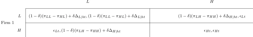
Just as in the Prisoner’s Dilemma example in section 2, we can use the one-stage deviation
principle to characterize the equilibrium of the infinitely repeated game as a Nash equilibrium
in the normal form game illustrated in figure 7 for every relevant history h and time t. Here,
ǫLt=ηLLt−ηHLt,ǫHt =ηHLt−ηHHt, ∆L|ht =vLL|ht−vHL|ht and ∆H|ht=vHL|ht−vHH|ht where
vij|htare equilibrium expected (with respect to the distribution ofη’s) average continuation payoffs.
Firm 1
Firm 2
L H
L (1−δ)(πLL−πHL) +δ∆L|ht,(1−δ)(πLL−πHL) +δ∆L|ht (1−δ)(πLH−πHH) +δ∆H|ht, ǫLt
H ǫLt,(1−δ)(πLH−πHH) +δ∆H|ht ǫHt, ǫHt
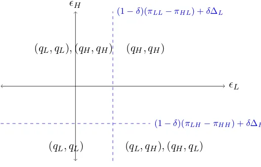
[image:17.612.70.560.527.599.2]ǫL
ǫH
(1−δ)(πLL−πHL) +δ∆L
(1−δ)(πLH−πHH) +δ∆H
(qH, qH)
(qL, qL),(qH, qH)
[image:18.612.170.434.132.301.2](qL, qL) (qL, qH),(qH, qL)
Figure 8: Nash equilibria of induced normal form
Since each of these normal form games depend on history h and timet, the Nash equilibria of
each of these games also depend on the realization of (ǫLt, ǫHt).7 Assume firms are only playing
pure strategies. Figure 8 summarizes the Nash equilibria of the normal form game in the (ǫLt, ǫHt)
space. For example, ifǫLt<(1−δ)(πLL−πHL) +δ∆L|ht and ǫHt <(1−δ)(πLH−πHH) +δ∆H|ht,
then the stage outcome (qL, qL) at timet, after historyh and upon observing these types ofǫ’s can
be sustained by some equilibrium strategy.
4.1 Data generation
Let the true marginal cost be equal toc0 = 0.5. I assume the the low and high quantities respectively
correspond to monopoly and Cournot quantities given by
qL=qM =
1−c0
4 =
1 8
qH =qC =
1−c0
3 =
1 6.
While firms are aware thatqL=qM and qH =qC, the econometrician doesnot have this
informa-tion. All the econometrician observes are the actual numerical values of qL and qH.
Instead of defining strategies explicitly, I simulate data directly by assuming ∆L=πM−πC and
∆H =πC−πC = 0 along the equilibrium path. Note that in a model with no shocks, i.e. ηij = 0,
these ∆’s are consistent with a Grim-Trigger strategy which would also imply Pr(qL, qL) = 1. This
need not be the case when there are shocks since outcomes such as (qH, qH) can occur along the
equilibrium path for certain values ofǫ’s and given properly defined strategies that are conditional
on ǫ’s.
I assume ǫ’s are independently distributed according to a logistic distribution with common
varianceσ2. Sinceǫ’s have full support, multiple equilibria in the normal form game given in figure 7
can arise depending on the realization of ǫ’s (see figure 8). This corresponds to the equilibrium
selection problem in static games (Tamer, 2003). I let s1 and s2 be static selection parameters
wheres1 is equal to the probability that (qL, qL) is chosen whenǫLt <(1−δ)(πLL−πHL) +δ∆L|ht
andǫHt>(1−δ)(πLH−πHH) +δ∆H|ht, whiles2 is equal to the probability that (qL, qH) is chosen
when ǫLt >(1−δ)(πLL−πHL) +δ∆L|ht and ǫHt <(1−δ)(πLH −πHH) +δ∆H|ht
Define individual choice probabilities as
p(∆;c) ≡ Pr (ǫL<(1−δ)(πLL−πHL) +δ∆|∆)
q(∆;c) ≡ Pr (ǫH <(1−δ)(πLH −πHH) +δ∆|∆).
The logistic distribution assumption impliestrue indidvidual choice probabilities being equal to
p0 ≡
exph(1−δ)(πLL−πHL)+δ∆L
σ
i
1 + exph(1−δ)(πLL−πHL)+δ∆L
σ
i
q0 ≡
exph(1−δ)(πLH−πHH)+δ∆H
σ
i
1 + exph(1−δ)(πLH−πHH)+δ∆H
σ
Finally observed frequencies of stage game outcomes are computed as:
Pr (qL, qL) = p0q0+s1·p0(1−q0)
Pr (qH, qH) = (1−p0)(1−q0) + (1−s1)·p0(1−q0)
Pr (qL, qH) = s2·(1−p0)q0
Pr (qH, qL) = 1−Pr (qL, qL)−Pr (qH, qH)−Pr (qL, qH).
I assume the econometrician observes (or knows or can estimate beforehand) the discount factor
δ, the inverse demand function P(Q), the distribution of the shocks including its varianceσ2, the
frequencies Pr (qL, qL), Pr (qH, qH), Pr (qL, qH) and Pr (qH, qL) and the actual values ofqL andqH.
The econometrician does not know the true marginal costc0, the static selection parameters (s1, s2),
the equilibrium continuation payoffs that are implemented, and finally thatqLand qH correspond
to the joint monopoly and Cournot quantities, respectively.
4.2 Identified set
The goal of the economectric exercise is to compute bounds for marginal cost and test for firm
conduct, i.e. H0 :qL=qM andH0:qL=qC. If both static and dynamic selection parameters were
known (i.e. s1, s2,∆L,∆H), then one can compute theoretical stage game frequencies as functions
of marginal cost, then find the value of marginal cost that best matches these with the observed
stage frequencies.8 Without this information, one can instead use the method in section 3 to get
an identified set for marginal cost.
The identification strategy requires knowing the extreme points of the set of equilibrium
con-tinuation payoffs. Instead of relying on a Folk Theorem for this modified repeated game, I impose
the restriction9 v
kk′ ∈[πC(c), πM(c)] whereπM(c) andπC(c) are individual firm’s (joint) Monopoly
8The “ample source of variation” in this case is the known distribution of shocks.
9Note that it is possible to have worse equilibrium punishments than the Cournot payoff using more complicated
strategies (Abreu, 1986; Abreu, 1988). I will derive the set of individually rational payoffs and use in a future version
and Cournot profits:
πM(c) = (1−c)
2
8 , π
C(c) = (1−c)2
9 .
These imply ∆(c) =πM(c)−πC(c) = (1−c)2/72 and ∆(c) =−∆(c). Finally, the identified set is the set of all values ofc that simultaneously satisfy the following:
Pr (qL, qL) ∈
p(∆(c))q(∆(c)), p ∆(c)
Pr (qH, qH) ∈
1−p ∆(c)
1−q ∆(c)
,1−q(∆(c))
Pr (qL, qH) ∈
0,(1−p(∆(c)))q ∆(c)
Pr (qH, qL) ∈
0,(1−p(∆(c)))q ∆(c)
4.3 Results
4.3.1 Bounds for marginal cost
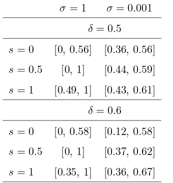
I compute the bounds for different values of the standard deviation of the logit profit shocks
σ (=1 and 0.001), discount factor δ (=1 and 0.001), and static selection parameters s1 and s2
(s1 =s2= 0,0.5,1). Table 1 contains the results. Since the inverse demand function isP = 1−Q,
[0,1] is a natural bound on marginal cost. Thus, the computed bounds are only informative if it is
a proper subset of [0,1].
The simulation parameter σ measures the standard deviation of the profit shocks. We can
interpret the magnitude ofσby comparing it to monopoly profits under the truec0 = 0.5, i.e. πM =
0.03125. Clearly, a standard deviation equal to one is large relative to profits, hence representing
an extreme case where decision-making will mostly be driven by these shocks. On the other hand,
a standard deviation of 0.001 represents about a 3% movement in monopoly profits. The estimated
bounds for marginal cost are much tighter whenσ is small. This reflects the fact that the incentive
compatibility constraints provide more information regarding outcomes when noise from exogenous
profits shocks are smaller.
Estimated bounds are also tighter when the discount factor δ is low. In this case, the incentive
compatibility constraints have more bite since collusion is harder to sustain with more impatient
firms. The valueδ = 0.5 is the lowest discount factor that will make Grim-Trigger an SPNE in the
game without profit shocks.
The static selection parameter sgives the probability that (qL, qL) and (qL, qH) are selected in
the induced normal form game (see figure 8). The bounds are tighter when s= 0.5 andσ smaller.
[image:22.612.224.397.313.496.2]Interestingly however, the bounds become uninformative withs= 0.5 whenσ is large.
Table 1: Bounds for marginal cost (c0 = 0.5)
σ= 1 σ= 0.001
δ= 0.5
s= 0 [0, 0.56] [0.36, 0.56]
s= 0.5 [0, 1] [0.44, 0.59]
s= 1 [0.49, 1] [0.43, 0.61]
δ= 0.6
s= 0 [0, 0.58] [0.12, 0.58]
s= 0.5 [0, 1] [0.37, 0.62]
s= 1 [0.35, 1] [0.36, 0.67]
4.3.2 Test of firm conduct
While the bounds on marginal cost are of interest themselves, they can also be used to provide
a test for firm conduct. Note that if we had a point estimate for marginal cost, we can compute
estimates of the monopoly and Cournot quantities ˆqM and ˆqC, respectively, predicted by theory.
However, since we only have bounds forcand not point estimates, we can only get bounds for these
predicted quantities. Nevertheless, these quantity bounds are still useful in determining whether
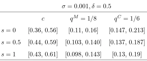
Table 2: Bounds for theoretical quantities
σ= 0.001, δ= 0.5
c qM = 1/8 qC = 1/6
s= 0 [0.36, 0.56] [0.11, 0.16] [0.147, 0.213]
s= 0.5 [0.44, 0.59] [0.103, 0.140] [0.137, 0.187]
s= 1 [0.43, 0.61] [0.098, 0.143] [0.13, 0.19]
Table 2 provides the bounds for marginal cost, and predicted monopoly and Cournot quantities
(based on theory).Considers= 0. Suppose we are interested in “testing”10 if the observed lowq
L
is consistent with qM orqC. In the data we observeq
L= 0.125. This value for the low quantity is
inside the identified set for qM and so we cannot reject that firms are colluding at the monopoly
quantity. On the other hand, qL= 0.125 is outside the identified set forqC and thus we can reject
that firms are competing in Cournot fashion. A similar test can be implemented for qH =qM and
qH = qC (observed qH = 0.167). Finally, the test has no power if identified set for c is too wide
(not very informative).
5
Extensions
The examples I discuss in the paper are simple enough such that it is easy to characterize the
set of equilibrium payoffs (or an non-trivial upper bound of it). In more complicated games, the
set of equilibrium payoffs are harder to compute. Nevertheless, methods have been developed to
compute equilibria in more complicated infinitely repeated games. For example, Judd, Yeltekin
and Conklin (2003) develop a computationally feasible algorithm to approximate the set of
equi-libria in infinitely repeated games with perfect monitoring and public randomization, following the
approach proposed by Abreu (1988), Abreu, Pearce and Stacchetti (1986, 1990), and Cronshaw
and Luenberger (1994). In on-going work, I explore how their method can be extended to games
without public randomization (nor mixed-strategies) using Milman’s converse to the Klein-Milman
theorem (see for example, Ok (2007)).
Finally, the method proposed in the paper can be adapted to dynamic games with states (i.e.
stochastic games), as long as the set of equilibrium continuation payoffs can be computed, or at
least its boundary. Dutta (1995) is an earlier attempt to compute equilibria in these games while
Yeltekin, Cai and Judd (2015) a more recent take on this problem.
References
Abreu, D. (1988), “On the Theory of Infinitely Repeated Games with Discounting,”Econometrica,
56 (2), 383-396.
Abreu, D., D. Pearce, and E. Stacchetti (1986), “Optimal Cartel Equilibria with Imperfect
Mon-itoring,”Journal of Economic Theory, 251-269.
Abreu, D., D. Pearce, and E. Stacchetti (1990), “Toward a Theory of Discounted Repeated Games
with Imperfect Monitoring,”Econometrica, 58 (5). 1041-1063.
Beresteanu, A., I. Molchanov, and F. Molinari (2011), “Sharp Identification Regions in Models
With Convex Moment Predictions,”Econometrica, 79 (6), 1785-1821.
Ciliberto, F. and E. Tamer (2009), “Market Structure and Multiple Equilibria in Airline Markets”,
Econometrica, 77 (6), 1791-1828.
Dal B´o, P. and G. R. Fr´echette (2011), “The Evolution of Cooperation in Infinitely Repeated
Games: Experimental Evidence,”American Economic Review, 101, 411-429.
Dutta, P. K. (1995), “A Folk Theorem for Stochastic Games,” Journal of Economic Theory, 66,
Cronshaw, M. and D. G. Luenberger (1994), “Strongly Symmetric Subgame Perfect Equilibrium in
Infinitely Repeated Games with Perfect Monitoring and Discounting,”Games and Economic
Behavior, 6, 220-237.
De Paula, A. (2013), “Econometric Analysis of Games with Multiple Equilibria”, Annual Review
of Economics, 5, pp. 107-131.
Fershtman, C. and Pakes, A. (2000), “A Dynamic Game with Collusion and Price Wars,”RAND
Journal of Economics, 31 (2), pp. 207-236.
Galichon, A. and Henry, M. (2011), “Set Identification in Models with Multiple Equilibria,”Review
of Economic Studies, 78 (4), pp. 1264-1298.
Green, E. J. and Porter, R. H. (1984), “Noncooperative Collusion Under Imperfect Price
Infor-mation,”Econometrica, 52 (1), pp. 87-100.
Judd, K. L., Yeltekin, S. and Conklin, J. (2003), “Computing Supergame Equilibria,”
Economet-rica, 71 (4), pp. 1239?1254.
Ok, E. A. (2007) Real Analysis with Economic Applications, Princeton: Princeton Univ Press.
Rotemberg, J. J. and Saloner, G. (1986), “A Supergame-Theoretic Model of Price Wars During
Booms,” American Economic Review, 76, pp. 390-407.
Tamer, E. (2003), “Incomplete Simultaneous Discrete Response Model with Multiple Equilibria’,”
Review of Economic Studies, 70, pp. 147?165.
Yeltekin, S., Cai, Y. and Judd, K.L. (2015), “Computing equilibria of dynamic games,” working