Munich Personal RePEc Archive
Semiparametric Efficient Adaptive
Estimation of the PTTGARCH model
Ciccarelli, Nicola
Tilburg University
2016
Online at
https://mpra.ub.uni-muenchen.de/72021/
Semiparametric Efficient Adaptive Estimation of the PTTGARCH model
Nicola Ciccarelli∗,
Tilburg University
Abstract
Financial data sets exhibit conditional heteroskedasticity and asymmetric volatility. In this paper we de-rive a semiparametric efficient adaptive estimator of a conditional heteroskedasticity and asymmetric volatility GARCH-type model (i.e., the PTTGARCH(1,1) model). Via kernel density estimation of the unknown density function of the innovation and via the Newton-Raphson technique applied on the√n-consistent quasi-maximum likelihood estimator, we construct a more efficient estimator than the quasi-maximum likelihood estimator. Through Monte Carlo simulations, we show that the semiparametric estimator is adaptive for parameters in-cluded in the conditional variance of the model with respect to the unknown distribution of the innovation.
JEL Classification: C14; C22.
Keywords: Semiparametric adaptive estimation; Power-transformed and threshold GARCH.
1
Introduction
Stock prices and other asset prices exhibit conditional heteroskedasticity, that is, volatility shocks are clustered
in some periods while other periods are characterized by low volatility. Engle (1982) proposed the ARCH model
to allow for the presence of conditional heteroskedasticity in asset prices. Bollerslev (1986) generalized Engle
(1982)’s idea with the GARCH(p,q) model. Additionally, Black (1976), Christie (1982), Engle (1990) and Engle
and Ng (1993) show that stock market prices are affected by asymmetric volatility. Essentially, the latter authors
show that stock prices tend to have higher volatility in the case of negative news than in the case of positive
news, leading to an asymmetric evolution of volatility through time. In order to capture the presence of volatility
asymmetry, many models were proposed starting with the Taylor-Schwert GARCH model [see Taylor (1986) and
Schwert (1989) for more details], the AGARCH(1,1) model proposed by Engle (1990) and the EGARCH model
proposed by Nelson (1991). One of the most recent asymmetric volatility models -i.e., the PTTGARCH(p,q)
model- was introduced by PWT (2008); the PTTGARCH(p,q) model is a very flexible model and, under certain
∗CentER and Department of Econometrics and Operations Research, Tilburg University, P.O. Box 90153, 5000 LE Tilburg, The
conditions, it includes several ARCH/GARCH models such as Bollerslev (1986)’s GARCH(p,q) model. Engle
and Ng (1993) and Awartani and Corradi (2005) compare the standard GARCH model with several asymmetric
GARCH-type models, and they conclude that asymmetric GARCH-type models are more appropriate than the
symmetric GARCH(1,1) model to forecast financial markets volatility.
Building upon these results we construct a semiparametric efficient adaptive estimator for the PTTGARCH
model, and, through a series of Monte Carlo simulations, we show that this estimator regains most of the efficiency
loss of the inefficient quasi-maximum likelihood estimator whenever the true innovation is not distributed as a
standard normal random variable or as a Gaussian mixture random variable. For simplicity we restrict our
attention to the PTTGARCH(1,1) model; anyhow, the results can be generalized to the PTTGARCH(p,q) case.
The paper is organized along the following lines. Section 2 contains two main results. First, we show that the
quasi-maximum likelihood estimator is consistent and asymptotically normal in the case of the PTTGARCH(1,1)
model. Second, we show that the log-likelihood ratio of the PTTGARCH(1,1) model satisfies the Local Asymptotic
Normality (LAN) condition. Through the Convolution theorem, the semiparametric estimator -which is built upon
the quasi-maximum likelihood estimator- is shown to achieve the semiparametric lower bound for the variance. In
Section 3 we show how to compute the theoretical asymptotic variance of the maximum likelihood (ML) and
quasi-maximum likelihood (QML) estimators in the case of the PTTGARCH(1,1) model. The theoretical asymptotic
variance of the maximum likelihood (ML) and quasi-maximum likelihood (QML) estimators are obtained through
simulation, and can be used to check whether Monte Carlo simulations are appropriately set up. In Section 4 we
report the results of Monte Carlo simulations; in this section we compare estimators in terms of their efficiency,
and we check whether the asymptotic results of the ML and QML estimators from Monte Carlo experiments
approximate well enough the theoretical asymptotic behavior of the ML and QML estimators. Section 5 concludes.
2
The Semiparametric Efficient Adaptive Estimator for the PTTGARCH(1,1)
model
The power-transformed and threshold GARCH(p, q) model [henceforth PTTGARCH(p, q) model] was introduced
by PWT (2008) [see equation (1.2) of PWT (2008), page 353], and it includes several conditional heteroskedasticity
models. In this paper we use the PTTGARCH(1,1) model without power-transformation, that is, we set δ = 1
and, for notational simplicity, we set p = 1 and q = 1 in equation (1.2) of PWT (2008). The PTTGARCH(1,1)
model used in this paper incorporates conditional heteroskedasticity and asymmetric volatility. Let{Yt}denote an
observed real-valued discrete-time stochastic process; the stochastic process{Yt}is conditionally heteroschedastic:
Yt=
p
where the unobservable heteroskedasticity factors {ht}t∈Z follow a PTTGARCH(1,1) process:
ht=ω+βht−1+α+(Yt+−1)2+α−(Yt−−1)2, (2.2)
where (and in the sequel) the notation [see Hwang and Kim (2004), page 296]
a+t = max(at,0) and a−t = max(−at,0) is used so thatat=a+t −a−t ,
and whereω >0,α+ ≥0,α− ≥0,β ≥0,h1= 1−β−1 ω 2(α+)−
1 2(α−)
.
It is not possible to obtain a semiparametric estimation of the PTTGARCH(1,1) model in eq. (2.1)-(2.2) that
is fully efficient since the score space is not orthogonal to the tangent space generated by the nuisance parameter
(i.e., the distribution of the standardized innovation), thus a reparametrization of the PTTGARCH(1,1) model
is needed to obtain a semiparametric efficient adaptive estimator. We set ω = 1 and we introduce the location
parameterµand the scale parameter σ in the PTTGARCH(1,1) model so that the orthogonality relation (3.6) of
DKW (1997) is satisfied.1
Letµ∈R,σ >0,α+>0,α−>0,β >0 be parameters2 and let{ηt:t∈Z}be an i.i.d. sequence of innovation
errors with zero mean, unit variance and densityf. Putξt=µ+σηt, thusξtis a random variable with location µ,
scaleσ and densityσ−1f({ξt−µ}/σ).Consider the reparametrized PTTGARCH(1,1) model with observations
Yt=
p
htξt=µ
p
ht+σ
p
htηt, ηt∼iid(0,1), (2.3)
where the unobservable heteroskedasticity factors {ht}t∈Z follow a PTTGARCH(1,1) process:
ht= 1 +βht−1+α+(Yt+−1)2+α−(Yt−−1)2 = 1 +ht−1
β+α+
ξ+t−12+α−ξt−−12
, (2.4)
where the notation [see Hwang and Kim (2004), page 296]
a+t = max(at,0) and a−t = max(−at,0) is used so thatat=a+t −a−t ,
where h1 = 1−1 1 2(α+)− 1 2(α−)−β
, and where α+ >0, α− >0, β >0,µ∈Rand σ >0.3 Observe that the Euclidean
parameterθ= (α+, α−, β, µ, σ)′ ∈Θ⊂R5 is identifiable.
1Similar reparametrizations are used in DK (1997) for the GARCH(1,1) model and in Sun and Stengos (2006) for the AGARCH(1,1)
model.
2From this point onwards in this paper, unless explicitly stated otherwise, we restrict our attention to the case of strictly positive
conditional variance parameters (i.e., α+ >0,α− >0,β > 0). We assume that parametersα+ andα− are strictly positive as it is
needed for the consistency of the quasi-maximum likelihood estimator [see Assumption QML4 in Section 2.4], and, for simplicity, we assume thatβis strictly positive.
We assume that the observed dataYtare stationary given the starting valueh1(θ) =h01initializing (2.4). The necessary and sufficient condition for a unique strictly stationary and ergodic solution for the (non-reparametrized)
PTTGARCH(1,1) model is reported in Liu (2006) [Theorem 2.1, page 1324]. We adapt the necessary and sufficient
condition given in Liu (2006) to the case of the reparametrized PTTGARCH(1,1) model.
Assumption 2.1. Strict Stationarity of the Reparametrized PTTGARCH(1,1) Model Based on The-orem 2.1 of Liu (2006)
E lnhβ+α+(ξt+)2+α−(ξ−t )2
i
<0. (2.5)
If Ehα+(ξ+t−k)2+α−(ξt−−k)2+β)i < 1, then the necessary and sufficient condition for the strict stationarity of
{ht:t∈Z}reported in eq. (2.5) is satisfied [see Assumption QML3 in Section 2.4 for the proof].
2.1 The Data Generating Process
We assume that there is an underlying probability distribution, or data generating process (DGP), for the
observ-able Yt and a true parameter vectorθ0 = (α0+, α0−, β0, µ0, σ0)′ which is a characteristic of that DGP, with
Yt=µ0 p
ht+σ0 p
htηt, ηt∼iid(0,1),
ht= 1 +β0ht−1+α0+(Yt+−1)2+α0−(Yt−−1)2 = 1 +ht−1
β0+α0+
ξt+−12+α0−
ξt−−12
,
wherea+t = max(at,0) anda−t = max(−at,0) is used so thatat=a+t −a−t [see Hwang and Kim (2004), page 296],
whereh1= 1−1 1 2(α+)− 1 2(α−)−β
, and whereα+>0,α− >0,β >0,µ∈Rand σ >0.
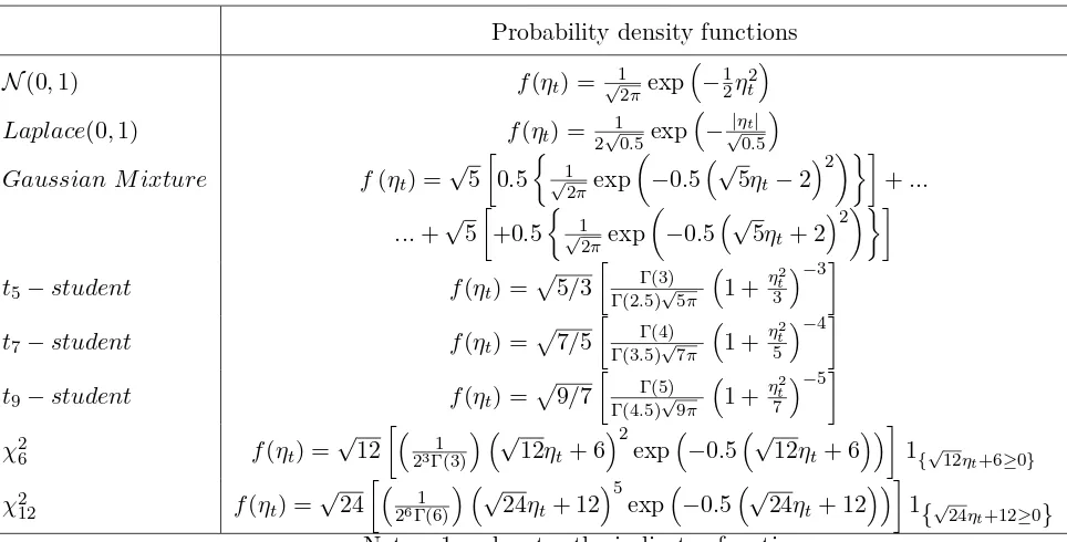
The probability density functions used for the innovationηt are: Normal(0,1), Laplace(0,1), Balanced Mixture
of two Normals, N(−2,1) and N(+2,1), t-student distributions with 5, 7, 9 degrees of freedom, Chi-squared
distributions with 6 and 12 degrees of freedom; all densities are rescaled so that the innovation has zero mean and
unit variance. The eight probability density functions for the standardized innovation ηtare reported in Table 1.
[Table 1]
2.2 The general form of the log-likelihood function of the PTTGARCH(1,1) model
The joint density function for a sampleY= (Y1, ..., YT) is the product of the conditional densities of{Yt:t= 2, ..., T}
and of the marginal density ofY1:
f(Y;θ) =f(Y1, ..., YT;θ) =f(YT|YT−1, ..., Y1;θ)×...
×f(YT−1|YT−2, ...Y1;θ)×...×f(Y2|Y1;θ)×f(Y1;θ)
Equation (2.6) can be rewritten as:
f(Y;θ) =
T
Y
t=2
f(Yt|It−1;θ)
!
f(Y1;θ)
where It = {Yt, ..., Y1} denotes the information available at time t, and Y1 denotes the initial value. The log-likelihood function may then be expressed as:
lnL(θ|Y) =
T
X
t=2
lnf(Yt|It−1;θ) + lnf(Y1;θ) (2.7)
The first term contained in eq. (2.7) is the conditional log-likelihood function while the second term in eq. (2.7)
is the marginal log-likelihood for the initial value. The marginal density of Y1 is dropped from the conditional likelihood function because its contribution is negligible when the number of observations is large, thus eq. (2.7)
can be rewritten as:
lnL(θ|Y) =
T
X
t=2
lnf(Yt|It−1;θ) (2.8)
Given eq. (2.3), for any t= 2, ..., T, the conditional density ofYt givenIt−1 =Yt−1, ..., Y1 is:
f(Yt|It−1;θ) = 1 σ√ht
f(ηt) = 1 σ√ht
f Yt−µ
√
ht σ√ht
!
(2.9)
Using (2.8) and (2.9), the conditional log-likelihood function is:
lnL(θ|Y) =
T
X
t=2
ln 1
σ√ht
f Yt−µ
√
ht σ√ht
!!
(2.10)
2.3 The log-likelihood function of the PTTGARCH(1,1) model for each type of innovation
Using the probability density functions reported in Table 1 and using eq. (2.10) we can obtain the conditional
log-likelihood function for each type of (zero mean and unit variance) innovationηt. The conditional log-likelihood
function for each type of (zero mean and unit variance) innovation is reported in Table 2.
[Table 2]
2.4 The Asymptotic Properties of the QML Estimator in the Case of the PTTGARCH(1,1)
Model
Hamadeh and Zako¨ıan (2011) prove that, under assumptions QML0-QML6 reported below, the quasi-maximum
likelihood estimator is consistent and asymptotically normal for the generic PTTGARCH(p,q) model in their
and asymptotic normality of the quasi-maximum likelihood estimator are satisfied in the case of the reparametrized
PTTGARCH(1,1) model studied in this paper. The consistency of the QML estimator is crucial to construct the
semiparametric efficient adaptive estimator; see Section 2.6 for more details. Assumptions QML0-QML6 reported below correspond to Assumptions A0-A6 of Hamadeh and Zako¨ıan (2011).
Assumption QML0. ηt is a sequence of independent and identically distributed (i.i.d.) random variables with E|ηt|r<∞ for some r >0.
First,ηtis generated as an i.i.d. random variable. Second,E|ηt|rcan be rewritten asE
q
η2
t
r
; choosingr = 2 we
obtain Eqη2t
r
=Eqη2t
2
=E ηt2
. Since the innovation has zero mean and unit variance by construction,
thenE ηt2
= 1<∞. Thus, Assumption QML0 is satisfied.
Assumption QML1. θ0 ∈Θ and Θis compact.
The vector of the true parameters in the PTTGARCH(1.1) model is:
θ0 = (α0+, α0−, β0, µ0, σ0)′
and belongs to a parameter space Θ⊂]0,∞[4×Rwith Θ compact since Θ is a bounded and closed set. Therefore, Assumption QML1 is satisfied.
Assumption QML2. Eη2
t = 1 and P[ηt > 0] ∈ (0,1). If P(ηt ∈ Γ) = 1 for a set Γ, then Γ has a cardinal
|Γ|>2.
Assumption QML2 is satisfied by construction: the (rescaled) innovation is created such that Eηt2 = 1 and such that the (rescaled) innovation includes both positive and negative values, thusP[ηt>0]∈(0,1). The cardinality
of the set Γ is|Γ|>2 since the innovationηtis generated as an i.i.d. random variable with a continuous probability
density function.
Assumption QML3. γ(A0)<0 and for all θ∈Θ,Ppj=1βj <1.
Assumption QML3 is satisfied if Ehα+(ξt+−k)2+α−(ξ−t−k)2+β
i
< 1. In order to show that Assumption QML3
is satisfied in the case of our model, we use the notation of Example 2.1 (GARCH(1,1)) of Francq and Zako¨ıan
(2010) [page 34], and we use other results presented in Chapter 2.2 of Francq and Zako¨ıan (2010).
Proof. In the PTTGARCH(1,1) model the matrixAtcan be written as [see Francq and Zako¨ıan (2010), page 34]
At= ((ξ+t )2,(ξt−)2,1)′(α+, α−, β).
We thus have
AtAt−1...A1 =
t−1 Y
k=1
It follows that
lnkAtAt−1...A1k=
t−1 X
k=1
ln(α+(ξt+−k)2+α+(ξt−−k)2+β) + lnkAtk.
The top Lyapunov exponent γ(A0) is defined as [see eq. (2.23) in Francq and Zako¨ıan (2010)]
γ(A0) = lim
t→∞a.s.
1
t lnkAtAt−1...A1k.
By the strong law of large numbers, the top Lyapunov exponent can be written as [see Francq and Zako¨ıan (2010),
page 34]
γ(A0) =Eln
α+(ξt+−k)2+α−(ξ−t−k)2+β
.
By the Jensen Inequality we obtain
γ(A0) =Eln
α+(ξt+−k)2+α−(ξt−−k)2+β
≤ lnhEα+(ξt+−k)2+α−(ξt−−k)2+β
i
.
Using the assumption Ehα+(ξt+−k)2+α−(ξt−−k)2+β
i
<1, we finally obtain
γ(A0) =Eln
α+(ξt+−k)2+α−(ξt−−k)2+β
≤lnEα+(ξt+−k)2+α−(ξ−t−k)2+β
<0
The second part of Assumption QML3 reduces in PTTGARCH(1,1) model to β < 1 and this assumption is
satisfied sinceγ(A0)<0 as shown above and α+>0 andα−>0 [see the restrictions below eq. (2.4)].
Let Aθ+(z) =Pqi=1αi+zi,Aθ−(z) =Pqi=1αi−zi and Bθ(z) = 1−Ppj=1βjzj. In the case of PTTGARCH(1,1)
model the previous equations simplify toAθ+(z) =α+z,Aθ−(z) =α−z andBθ(z) = 1−βz.
Assumption QML4. If p > 0, Bθ0(z) has no common root with Aθ0+(z) and Aθ0−(z). Moreover Aθ0+(1) +
Aθ0−(1)6= 0 andα0++α0−+β06= 0.
Assumption QML4 is satisfied. Aθ0+(1) +Aθ0−(1)6= 0 is verified sinceα0+ >0 andα0−>0. The root ofAθ0+(z)
is:
Aθ0+(z) = 0 =α0+z⇒z= 0.
The root ofAθ0−(z) is:
Aθ0+(z) = 0 =α0−z⇒z= 0.
and Bθ0(0)6= 0. Ifβ0 6= 0, the unique root of Bθ0(z) is:
The unique root of Bθ0(z) is 1/β0 > 0 (if β0 = 0, the polynomial does not admit any root) and because the
coefficients α0+ and α0− are positive, Aθ0+(1/β0)6= 0 and Aθ0−(1/β0)6= 0.
Given the above results, α0++α0−+β06= 0.
Theorem 2.1.[Hamadeh and Zako¨ıan (2011)] Let (ˆθnQM L) be a sequence of QML estimators satisfying (2.1) of Hamadeh and Zako¨ıan (2011). Then, under assumptions QML0-QML4, θˆQM Ln →θ0, a.s. as n→ ∞.
Proof. See Hamadeh and Zako¨ıan (2011), Proof of Theorem 2.1, pages 497-499.
Two additional assumptions are needed for the asymptotic normality of the QML estimator.
Assumption QML5. θ0 ∈Θ˙, where Θ˙ denotes the interior ofΘ.
Assumption QML5 is satisfied: if ˆθn is consistent, it also belongs to the interior of Θ, for largen.
Assumption QML6. κη :=Eηt4<∞.
Assumption QML6 is satisfied since the kurtosis of each (zero mean and unit variance) innovationηtis finite; see
Table 3 for the kurtosis of each innovation.
[Table 3]
Theorem 2.2.[Hamadeh and Zako¨ıan (2011)] Under assumptions QML0-QML6,
√
nθˆnQM L−θ0
⇒ N(0,(κη−1)J−1),
where J =Eθ0 ∂2ℓ
t(θ0)
∂θ∂θ′
= 4Eθ0
1
h2
t(θ0)
∂ht(θ0)
∂θ
∂ht(θ0)
∂θ′
.
Proof. See Hamadeh and Zako¨ıan (2011), Proof of Theorem 2.2, pages 499-502.
2.5 Local Asymptotic Normality and the Convolution Theorem
Let µ∈R, σ >0, α+>0, α− >0, β >0 be parameters4 and let {ηt:t∈Z} be an i.i.d. sequence of innovation
errors with zero mean, unit variance and densityf. Put ξt=µ+σηt, thusξt is a random variable with location
µ, scaleσ and density σ−1f({ξt−µ}/σ).
Consider the reparametrized PTTGARCH(1,1) model with observations
Yt=
p
htξt=µ
p
ht+σ
p
htηt, ηt∼iid(0,1), (2.11)
where the unobservable heteroskedasticity factors {ht}t∈Z follow a PTTGARCH(1,1) process:
ht= 1 +βht−1+α+(Yt+−1)2+α−(Yt−−1)2 = 1 +ht−1
β+α+
ξ+t−12+α−ξt−−12
, (2.12)
where the notation [see Hwang and Kim (2004), page 296]
a+t = max(at,0) and a−t = max(−at,0) is used so thatat=a+t −a−t ,
where h1 = 1−1 1 2(α+)− 1 2(α−)−β
, and whereα+>0, α−>0, β > 0,µ∈ Rand σ >0. Observe that the Euclidean
parameter θ = (α+, α−, β, µ, σ)′ ∈ Θ ⊂ R5 is identifiable. The necessary and sufficient condition for a unique
strictly stationary solution {ht:t∈Z} is reported in Assumption 2.1.
In this section we show that the log-likelihood ratio of the PTTGARCH(1,1) model in (2.11)-(2.12) satisfies
theLocal Asymptotic Normality condition defined in Theorem 2.5.1 below. This condition was introduced by Le
Cam (1960), and it requires that, in large samples, the log-likelihood ratio is approximately quadratic in a small
neighborhood of the true parameter [Linton (1993)]. The LAN condition is necessary to establish the properties of
the semiparametric estimator presented in Section 2.6; Fabian and Hannan (1982) show that if the log-likelihood
ratio satisfies the LAN condition, then theLocal Asymptotic Minimax bound is achieved by estimators equivalent
to the MLE [Linton (1993)].
Le Cam (1960), Swensen (1985) and Roussas (1979) give conditions under which the log-likelihood ratio
of a general stochastic process satisfies the LAN condition [Linton (1993)]; these conditions have been verified
for stationary ARMA processes by Kreiss (1987), and DKW (1997) generalized the results of Kreiss (1987) to
classes of non-linear time-series (location-scale) models [Wellner et al. (2006)]. In this paper, following DKW
(1997), we show that the LAN property holds in the case of the reparametrized PTTGARCH(1,1) model as the
reparametrized PTTGARCH(1,1) model is a non-linear time-series (location-scale) model that satisfies conditions
in DKW (1997). Following DKW (1997), we also give the relevant assumptions such that semiparametric efficient
adaptive estimation is possible forπ = (α+, α−, β).
In order to derive asymptotic results, we assume that the observed data Y1,...,Yn are stationary given the
starting value h1(θ) =h01 initializing equation (2.12); this is insured by Assumption 2.1. The parameter vector
θ can be estimated based on h01,Y1,...,Yn, in the presence of the infinite-dimensional nuisance parameter f. We
fix the nuisance parameter f in this section,5 and we show that the resulting parametric model satisfies the LAN (Local Asymptotic Normality) property. Finally, we derive a bound on the asymptotic performance of regular
estimators of θ (ie., the Convolution Theorem).6
5On the contrary, in section 2.6 the nuisance parameterf(η
t) is unknown and is estimated using the kernel density estimator.
Observe that if we also fix α+, α−, β, then our model is the location-scale model for i.i.d. random variables
[DK (1997)]; thus, the location-scale model is a parametric submodel of our time-series model and it is reasonable
to assume that this submodel is regular [DK (1997)],7 i.e.:
Assumption 2.2. f is an absolutely continuous Lebesgue density function with first order derivativef′ and finite
Fisher information for location
Il(f) =
Z f′
f
2
f(η)dη <∞, (2.13)
and finite Fisher information for scale:
Is(f) =
Z
1 +ηf′ f
2
f(η)dη <∞. (2.14)
Furthermore, the random variable η has location zero and scale one.
In order to derive the local asymptotic normality results of an estimator, we need a sequence of non-stochastic
values θn = (αn+, αn−, βn,µn, σn)′ and ˜θn = ( ˜αn+,α˜n−, ˜βn,µ˜n,˜σn)′ near the true parameter vector θ0 = (α0, β0, γ0, µ0, σ0)′ such that |θn−θ0|= O(n−1/2),|θ˜n−θ0|= O(n−1/2), and even
λn=√n
˜
θn−θn
→λ, asn→ ∞. (2.15)
In the rest of this section expectations, convergences, etc. are implicitly taken under θn and f.
In order to obtain a uniform LAN theorem we consider the log-likelihood ratio Λnofh01,Y1,...,Ynfor ˜θnwith
respect toθn underθn (andf fixed). To derive the joint density ofY1,...,Yn, usingh1(θ) =h01, we calculate the residuals and conditional variances recursively fort= 1,2, ...
ξt(θ) = Yt
p
ht(θ)
, (2.16)
ηt(θ) =
ξt(θ)−µ
σ , (2.17)
ht+1(θ) = 1 +βht(θ) +α+(Yt+)2+α−(Yt−)2. (2.18)
The density of Y1,..., Yn underθn, conditionally on h01, is
n
Y
t=1
σ−n1h−
1/2
nt f(σ−
1
n
n
h−nt1/2Yt−µn
o
) = n
Y
t=1
σn−1h−
1/2
nt f({ξnt−µn}/σn) = n
Y
t=1
σ−n1h−
1/2
nt f(ηnt), (2.19)
wherehnt=ht(θn),ξnt =ξt(θn) and ηnt =ηt(θn).
To emphasize the link between the present time-series model and the i.i.d. location-scale model we introduce
the notation ˜hnt =ht(˜θn),
l{µ, σ}(x) = log f({x−µ}/σ)−logσ,
Mnt
Snt
=n
1/2σ−1
n h−
1/2
nt
˜
µn˜h1nt/2−µnh1nt/2
˜
σn˜h1nt/2−σnh1nt/2
, (2.20)
and ˜ηnt =ηt(˜θn). Denoting the log-likelihood ratio for the initial value h01 as Λsn, we can write the log-likelihood
ratio Λnas
Λn= log
( n Y
t=1 ˜
σn−1˜hnt−1/2f(˜ηnt)/ n
Y
t=1
σ−n1h−nt1/2f(ηnt)
)
+ Λsn=...
=
n
X
t=1
{ℓ{(µn, σn) +σnn−1/2(Mnt, Snt)}(ξnt)−ℓ{µn, σn}(ξnt)}+ Λsn=...
=
n
X
t=1
{ℓ{(0,1) +n−1/2(Mnt, Snt)}(ηnt)−ℓ{0,1}(ηnt)}+ Λsn. (2.21)
Equation (2.21) is similar to the log-likelihood ratio statistic for the i.i.d. location-scale model but the deviations
Mnt and Snt are random in equation (2.21); in the following discussion we will apply the results of DKW (1997)
which allow for such random sequences.
To eliminate asymptotically the dependence of the log-likelihood ratio statistic on the initial value h01, we will use the following regularity condition [see Assumption A in DKW (1997)].
Assumption 2.3. The density fθ of the initial value h01 satisfies, under θn,
Λsn= log{fθ˜n(h01)/fθn(h01)}
P
→0 asn→ ∞. (2.22)
In order to make an expansion of Λn, we introduce the notation ˙ℓnt for the five-dimensional conditional score
at timet. Denote the three-dimensional vector derivative of the conditional variance by
Ht(θ) = ∂ht(θ) ∂(α+, α−, β)
=βHt−1(θ) +
(Yt+−1)2 (Yt−−1)2
ht−1(θ)
, (2.23)
with H1(θ) = 03. Define the (5×2)-derivative matrix Wt(θ) -which is motivated by differentiation of (Mnt, Snt)
with respect to ˜θn atθn- by
Wt(θ) =σ−1
1 2h−
1
t (θ)Ht(θ)(µ, σ)
I2
whereI2 is the (2×2) identity matrix. Denote the location-scale score by
ψt(θ) =−
f′(ηt(θ))
f(ηt(θ))
1 +ηt(θ)f
′(ηt(θ))
f(ηt(θ))
=−
ℓ′(ηt(θ))
1 +ηt(θ)ℓ′(ηt(θ))
, (2.25)
where we denoteℓ′ = ff′, and put
˙
ℓt(θ) =Wt(θ)ψt(θ).
Using the previous notation, the conditional score at time t can be denoted by ˙ℓnt = ˙ℓt(θn). An expansion of
(2.21) shows that the log-likelihood ratio Λn can be written as
Λn=λ′n−1/2 n
X
t=1 ˙
ℓnt−
1 2n
−1Xn
t=1
{λ′ℓ˙nt}2+Rn. (2.26)
In Appendix B we show that the following LAN theorem [Theorem 2.1 of DKW (1997)] holds for the parametric
version of model (2.11),(2.12).
Theorem 2.5.1. LAN
Suppose that Assumptions 2.1, 2.2, 2.3 are satisfied. Then the local log-likelihood ratio statistic Λn, as defined by
(2.21) and by (2.26)is asymptotically normal. More precisely, under θn,
Rn→P 0, Λn→D N(−
1 2λ
′I(θ0)λ, λ′I(θ0)λ) asn→ ∞, (2.27)
where I(θ0) is the probability limit of the averaged score products ℓ˙ntℓ˙′nt.
Proof. See Appendix B.
This LAN theorem implies that the sequences of probability measures {Pθn,f} and {Pθ˜n,f} are contiguous. We
can now apply the Convolution Theorem of H´ajek (1970) [see Theorem 2.3.1 of BKRW (1993)].
Theorem 2.5.2. Convolution Theorem
Under the assumptions of the LAN Theorem 2.5.1, let {Tn:n∈N} be a regular sequence of estimators of q(θ),
where q:R5 →Rk is differentiable with total differential matrix q˙. As usual, regularity at θ=θ0 means that there
exists a random k-vector Z such that for all sequences {θn:n∈N}, withn1/2(θn−θ0) = O(1),
where the convergence is under θn. Let ℓ˜= ˙q(θ0)I(θ0)−1ℓ˙(θ0) be the efficient influence function, then, under θ0,
n1/2{T
n−q(θ0)−n−1Pnt=1ℓ˜t} n−1/2Pn
t=1ℓ˜t
D
→
∆0
Z0
asn→ ∞, (2.29)
where ∆0 and Z0 are independent and Z0 is N(0,q˙(θ0)I(θ0)−1q˙(θ0)′). Furthermore, {Tn:n∈N} is efficient if
{Tn:n∈N} is asymptotically linear in the efficient influence function, i.e. if∆0 = 0 (a.s.).
From the Convolution Theorem we obtain that a regular estimator ˆθnofθsatisfies, underθ0,√n(ˆθn−θ0)→D ∆0+Z0, that is, the limit distribution of ˆθn is the convolution of the random vector ∆0 and a Gaussian random vector
Z0 with mean zero and variance equal to the inverse of the information matrix I(θ0) (ie., the Cramer Rao lower bound).
2.6 The Semiparametric Efficient Adaptive Estimator
Our approach follows DK (1997), who derive a semiparametric efficient adaptive estimator for the GARCH(1,1)
model while we derive a semiparametric efficient adaptive estimator for the (reparametrized) PTTGARCH(1,1)
model.
In semiparametric models there exist methods to upgrade √n-consistent estimators to efficient ones using the
Newton-Raphson technique as long as it is possible to accurately estimate the relevant score or influence functions.
In Schick (1986) such a method based on “sample splitting” and Le Cam’s “discretization” is described for i.i.d.
models [DK (1997)]. DKW (1997) adapted Schick (1986)’s method to the case of time-series models [see Theorem
3.1 of DKW (1997)]. Following DK (1997), we apply the discretization ofθn and the sample splitting method in
our proofs.8 If a √n-consistent estimator is available, it is trivial to derive the discretized local parameters near
θ0 since for any subsequence of{θˆn}, there are{θˆnk}satisfying the condition (2.15) [Sun and Stengos (2006)]. We
assume the existence of a preliminary, √n-consistent estimator.
Assumption 2.4. There exists a √n-consistent estimator θˆn of θn (under θn and f).
For our (reparametrized) PTTGARCH(1,1) model a natural candidate for such an initial estimator is the QML
estimator; see Section 2.4 for the √n-consistency and asymptotic normality of the QML estimator in the case of
the PTTGARCH(1,1) model.
We focus on efficient and adaptive estimation of the parameters α+, α−, β.9 Theorem 3.1 of DKW (1997)
contains the assumptions that are needed to obtain adaptive estimation in time-series models. In Appendix C we
verify the conditions of Theorem 3.1 of DKW (1997), this yields the following theorem.
8The sample splitting method is introduced as a technical tool that simplifies the proofs.
9Alternatively, in view of eq. (2.24), note that the score ˙ℓ
Theorem 2.6.1. Under Assumptions 2.1, 2.2, 2.3, 2.4 adaptive estimators of α+, α−, β do exist.
Proof. See Appendix C.
Let ˆθn=
ˆ
αn+,αˆn−,βˆn,µˆn,σˆn
′
be the√n-consistent estimator ofθand computeWt(ˆθn) via (2.23) and (2.24).
Let ˆηn1, ....,ηˆnnbe the residuals computed fromh1, Y1, ...., Ynand ˆθnusing (2.17). Based on the estimated residuals
ˆ
ηn1, ....,ηˆnn, we estimate nonparametricallyf(·) using the kernel density estimator with the standardized normal
kernelK(·) and bandwidthbn:10
ˆ
fn(·) =
1
n n
X
t=1 1
bn K
· −ηˆnt bn
,
and subsequently we estimateψ(·) by ˆψn(·);11 here bn→0 and nb4n → ∞. Our semiparametric estimator can be
written as
ˆ
αn+,αˆn−,βˆn
′
+ (I3,02×2) 1
n n
X
t=1
Wt(ˆθn) ˆψn(ˆηnt) ˆψn(ˆηnt)′Wt(ˆθn)′
!−1
×...
× 1
n n
X
t=1 (
Wt(ˆθn)−
1
n n
X
s=1
Ws(ˆθn)
) ˆ
ψn(ˆηnt), (2.30)
where ˆθn is the QML estimator. This is the semiparametric estimator used in the simulations of Section 4. We
need the following two technical modifications in order to prove that the semiparametric estimator is adaptive.
Discretization ˆ
θnis discretized by changing its value in (0,∞)×(0,∞)×(0,∞)×R×(0,∞) into one of the nearest points in the
grid √cn(N× N× N× Z× N). This method gives the possibility to consider ˆθn to be non-random, and therefore
independent of ˆηnt,Yt and h1 [DK (1997)]. Sample splitting
The set of residuals ˆηn1, ...,ηˆnn is split into two samples, which may be viewed as independent [DK (1997)]. For
ˆ
ηnt in the first sample, the second sample is used to estimateψ(·) by ˆψn2(·), and ˆψn(ˆηnt) in eq. (2.30) is replaced
by ˆψn2(ˆηnt); for ˆηnt in the second sample, the first sample is used to estimate ψ(·) by ˆψn1(·), and ˆψn(ˆηnt) in eq.
(2.30) is replaced by ˆψn1(ˆηnt).
10The kernel functionK(
·) used in our study is the standardized normal kernel: K ·−ˆηnt
bn
= √1 2πexp
−0.5 ·−ηˆnt
bn 2
.
11The kernel density derivative estimator can be written as [Wand and Jones (1995), page 49]: ˆf′
n(·) = n1
Pn t=1
1
b2
nK
′ ·−ηˆnt
bn
,
where K′(·) is the derivative of the standard normal density function. Finally, the location-scale score can be estimated using
ˆ
ψn(·) =−
" fˆ′ n(·) ˆ
fn(·)
1 + ˆηt
ˆ
fn′(·) ˆ
fn(·). #
3
The Theoretical Asymptotic Variance of the ML and the QML Estimators
3.1 The Theoretical Asymptotic Variance of the ML Estimator
In this sectionWt(·),ht(·),Ht(·),ψt(·) are evaluated at the true parameters (θ0). In the Monte Carlo experiments
for the PTTGARCH(1,1) model, the parameterµis set to zero and is not estimated [see Section 4], thus eq. (2.25)
becomes
ψt(θ0) =−
1 +ηt(θ0)
f′(ηt(θ0)) f(ηt(θ0))
, (3.1)
and eq. (2.24) becomes
Wt(θ0) =
1
2h−t1(θ0)Ht(θ0)
σ0−1
=
1
2h−t1(θ0)∂h∂αt(+θ0)
1
2h−t1(θ0)∂h∂αt(−θ0) 1
2h−t1(θ0)∂h∂βt(θ0)
σ0−1
, (3.2)
where the three-dimensional vector of derivativesHt(θ0) -reported in eq. (2.23)- is evaluated at the true parameters (θ0). The analytical solution for ψt(θ0) for each type of innovation is reported in Appendix A. The Fisher information matrix can be written as
I(θ0) =Is(f)E(Wt(θ0)Wt(θ0)′), (3.3)
withIs(f) denoting the Fisher information for scale described by
Is(f) =E[ψt(θ0)ψt(θ0)] =E
1 +ηt(θ0)
f′(η
t(θ0))
f(ηt(θ0))
2 =
Z
1 +ηt(θ0)
f′(η
t(θ0))
f(ηt(θ0))
2
f(ηt(θ0))dηt.
The Fisher information for scale is computed by numerical integration for each type of innovation and is reported
in Table 4.
[Table 4]
The Fisher information matrix reported in eq. (3.3) can be written as
×
Eθ0 1 4ht(θ0)2
∂ht(θ0)
∂α+
∂ht(θ0)
∂α+
1 4ht(θ0)2
∂ht(θ0)
∂α+
∂ht(θ0)
∂α−
1 4ht(θ0)2
∂ht(θ0)
∂α+
∂ht(θ0)
∂β ht0(.θ50)
∂ht(θ0)
∂α+
1 4ht(θ0)2
∂ht(θ0)
∂α−
∂ht(θ0)
∂α+
1 4ht(θ0)2
∂ht(θ0)
∂α−
∂ht(θ0)
∂α−
1 4ht(θ0)2
∂ht(θ0)
∂α−
∂ht(θ0)
∂β
0.5
ht(θ0)
∂ht(θ0)
∂α−
1 4ht(θ0)2
∂ht(θ0)
∂β
∂ht(θ0)
∂α+
1 4ht(θ0)2
∂ht(θ0)
∂β
∂ht(θ0)
∂α−
1 4ht(θ0)2
∂ht(θ0)
∂β
∂ht(θ0)
∂β ht0(.θ50)
∂ht(θ0)
∂β
0.5
ht(θ0)
∂ht(θ0)
∂α+
0.5
ht(θ0)
∂ht(θ0)
∂α−
0.5
ht(θ0)
∂ht(θ0)
∂β 1 .
The (4x4)-dimensional matrix E(Wt(θ0)Wt(θ0)′) -reported in eq. (3.3)- is computed through simulation. The theoretical asymptotic variance matrix of the MLE can be written as
V0=
[I(θ0)]−1
N , (3.4)
where N is the dimension of the sample (i.e. N=2000). In order to estimate the asymptotic variance of the
MLE, the number of time periods used is N=2000 and 5000 replications are used.12 The theoretical standard deviations ˆσα+, ˆσα− and ˆσβ are obtained by taking the square root of (the diagonal elements of)V0 [see eq. (3.4)].
The theoretical asymptotic standard deviations ˆσα+, ˆσα− and ˆσβ are reported in Table 5 for each combination of
(α+, α−, β) [see Section 4].
3.2 The Theoretical Asymptotic Variance of the QML Estimator
All vectors and matrices used in this section are evaluated at the true parameters (θ0). In the Monte Carlo experiments for the PTTGARCH(1,1) model, the parameterµ is set to zero and is not estimated, thus the score
becomes a (4×1) vector ˙ℓt(θ0) =Wt(θ0)ψt(θ0), withψt(θ0) reported in eq. (3.1) andWt(θ0) reported in eq. (3.2).13 The theoretical asymptotic variance of the QML estimator can be written as
V0 =
J(θ0)−1I(θ0)J(θ0)−1
N ,
where I(θ0) is the Fisher information matrix evaluated atθ0 and J(θ0) is the negative of the expectation of the Hessian evaluated at θ0:
I(θ0) =Eθ0 ∂l
t(θ0)
∂θ
∂lt(θ0)
∂θ
,
J(θ0) =−Eθ0
∂2lt(θ0) ∂θ∂θ
!
.
12Firstly, the asymptotic variance of the MLE was estimated with 2500 replications and with 5000 replications; the two estimations
gave slightly different results, thus the estimation of the asymptotic variance of the MLE with 5000 replications was adopted in order to obtain more precise estimates. Second, we obtained approximately the same (estimated) asymptotic variance of the MLE using a higher number of replications than 5000 replications, thus the choice of 5000 replications for the estimation of the asymptotic variance of the MLE was retained.
13ℓ˙
The theoretical asymptotic variance matrix of the QMLE can be written as
V0 = J(θ0)
−1I(θ0)J(θ0)−1
N =
1
N
(κη−1)
2 ×...
×
Eθ0 1 2ht(θ0)2
∂ht(θ0)
∂α+
∂ht(θ0)
∂α+
1 2ht(θ0)2
∂ht(θ0)
∂α+
∂ht(θ0)
∂α−
1 2ht(θ0)2
∂ht(θ0)
∂α+
∂ht(θ0)
∂β ht(1θ0)
∂ht(θ0)
∂α+
1 2ht(θ0)2
∂ht(θ0)
∂α−
∂ht(θ0)
∂α+
1 2ht(θ0)2
∂ht(θ0)
∂α−
∂ht(θ0)
∂α−
1 2ht(θ0)2
∂ht(θ0)
∂α−
∂ht(θ0)
∂β ht(1θ0)
∂ht(θ0)
∂α−
1 2ht(θ0)2
∂ht(θ0)
∂β
∂ht(θ0)
∂α+
1 2ht(θ0)2
∂ht(θ0)
∂β
∂ht(θ0)
∂α−
1 2ht(θ0)2
∂ht(θ0)
∂β
∂ht(θ0)
∂β ht(1θ0)
∂ht(θ0)
∂β
1
ht(θ0)
∂ht(θ0)
∂α+
1
ht(θ0)
∂ht(θ0)
∂α−
1
ht(θ0)
∂ht(θ0)
∂β 2 −1 , (3.5)
where N is the dimension of the sample (i.e., N = 2000) and where κη is the innovation’s kurtosis. The kurtosis
of each type of innovation is reported in Table 3. We compute the asymptotic variance of the QMLE through
simulation using 5000 replications.14 Taking the square root of (the diagonal elements of)V0 [see eq. (3.5)], the theoretical standard deviations ˆσα+, ˆσα− and ˆσβ are obtained. The theoretical asymptotic standard deviations
ˆ
σα+, ˆσα− and ˆσβ are reported in Table 5 for each combination of (α+, α−, β) [see Section 4].
4
Monte Carlo Experiments
To enhance the interpretation and validity of the theoretical results of the previous sections we present Monte Carlo
experiments in this section. The main purpose of Monte Carlo experiments is to evaluate the moderate sample
properties of the QMLE, MLE and the semiparametric estimator. The sample size for Monte Carlo experiments
isN = 2000. This choice is made since in the case of the PTTGARCH(1,1) model, two parameters (i.e., α+,α−)
are estimated using approximately half of the sample size [see Section 2 for more details].15
The number of replications used in each Monte Carlo experiment is equal to 2500 as in DK (1997) and in recent
studies [e.g., Pakel et al. (2011)]. Diaz-Emparanza (2002) studies the effect of the number of replications on the
accuracy of Monte Carlo experiments; the author shows that 1000 (or less than 1000) replications yield a low level
of accuracy of Monte Carlo experiments as the empirical distribution of estimated parameters obtained through
Monte Carlo experiments is quite different from the theoretical distribution. Since we choose 2500 replications
for our Monte Carlo experiments, the problems outlined in Diaz-Emparanza (2002) are unlikely to apply in our
context.
14Firstly, the asymptotic variance of the QMLE was estimated with 2500 replications and with 5000 replications; the two estimations
gave slightly different results, thus the estimation of the asymptotic variance of the QMLE with 5000 replications was adopted in order to obtain more precise estimates. Second, we obtained approximately the same (estimated) asymptotic variance of the QMLE using a higher number of replications than 5000 replications, thus the choice of 5000 replications for the estimation of the asymptotic variance of the QMLE was retained.
15Additionally, semiparametric estimators tend to yield strong efficiency improvements with respect to the QMLE in the case of
Monte Carlo experiments are conducted using the data generating process described in Section 2.1. The
con-ditional mean parameter µ is set to zero and is not included in the set of estimated parameters since our main
interest is in the estimation of the conditional variance parameters (α+, α−, β). The choice of setting µ= 0 is not
uncommon in studies that construct semiparametric estimators for conditional heteroskedasticity models; for
ex-ample, DK (1997) set the conditional mean parameter equal to zero and Sun and Stengos (2006) set the conditional
mean parameter to a value that is very close to zero. Three combinations for the set of parameters (α+, α−, β, σ)
are used in Monte Carlo experiments: (α+, α−, β, σ) = (0.20,0.40,0.60,1), (α+, α−, β, σ) = (0.075,0.15,0.80,1),
(α+, α−, β, σ) = (0.08,0.11,0.87,1); we choose these combinations of parameters (α+, α−, β, σ) to check the
per-formance of the semiparametric estimator as persistence of the PTTGARCH process increases.16
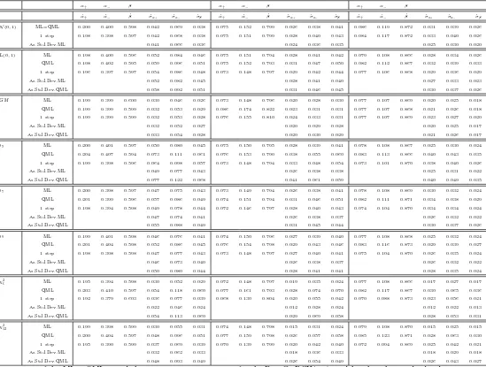
The sample means and sample standard deviations of the estimates obtained from Monte Carlo experiments
using the MLE, QMLE and the semiparametric estimator are reported in Table 5. The sample means and sample
standard deviations of the estimates using the MLE are reported in order to confront the efficiency of the
semi-parametric estimator with the MLE, even though the consistency and the asymptotic normality of the MLE was
not proved for the PTTGARCH(1,1) model. Additionally, the theoretical asymptotic standard deviations ˆσα+,
ˆ
σα−, ˆσβ, obtained with the estimation of the theoretical asymptotic variance of the MLE and QMLE [see Section
3], are added to Table 5 in order to check whether the asymptotic results of the MLE and QMLE from Monte
Carlo experiments approximate well enough the theoretical asymptotic behavior of the MLE and QMLE. In the
semiparametric part we used the standardized normal kernel with a bandwidth ofh= 0.40; reasonable changes of
the bandwidth, say 0.30≤h≤0.50 do not alter the conclusions below.
This section is organized in the following way: (1) in order to check whether the asymptotic results of the Monte Carlo experiments approximate the theoretical asymptotic behavior of the MLE and QMLE, in Section
4.1 the theoretical asymptotic standard deviations ˆσα+, ˆσα−, ˆσβ of the MLE and QMLE are compared with the
standard deviations of the MLE and QMLE obtained from Monte Carlo experiments. In order to have an easier
comparison between theoretical asymptotic results and Monte Carlo results, the asymptotic relative efficiencies
(AREs) of the MLE and QMLE are compared with the relative efficiencies (REs) of the MLE and QMLE in the
same section. (2) The main results of this section are reported in Section 4.2. In this section, the performance of the MLE, QMLE and the semiparametric estimator is evaluated through the relative efficiencies (REs) of the
estimators. (3)Some considerations and remarks are reported in Section 4.3.
[Table 5]
16Furthermore, we choose these combinations of parameters (α
+, α−, β, σ) to insure that the PTTGARCH process does not
4.1 Comparison of the Standard Deviations from the Monte Carlo Experiments with the
Theoretical Asymptotic Standard Deviations
The standard deviations of the MLE ˆσα+, ˆσα− and ˆσβ obtained from Monte Carlo experiments are close to the
theoretical asymptotic standard deviations of the MLE [Table 5]. Also, the standard deviations of the QMLE ˆσα+,
ˆ
σα− and ˆσβ obtained from Monte Carlo experiments are close to the theoretical asymptotic standard deviations
of the QMLE [see Table 5]. As a consequence, the asymptotic relative efficiencies (AREs) of the QMLE versus
the MLE are close to the relative efficiencies (REs) of the QMLE versus the MLE [compare Table 6 with Table 7].
To conclude, the asymptotic results of the MLE and QMLE from Monte Carlo experiments seem to approximate
well enough the theoretical asymptotic behavior of the MLE and QMLE.
[Table 6]
[Table 7]
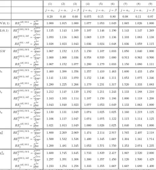
4.2 The Relative Efficiencies of the Estimators
The performance of the three estimators used in Monte Carlo experiments is evaluated through the relative
efficiencies (REs) of the estimators which are reported in Table 7.
In the case of the N(0,1)innovation, we only compare the semiparametric estimator with the MLE since the
QMLE is equivalent to the MLE in this case. The semiparametric estimator is almost as efficient as the MLE.
For the Laplace(0,1) innovation, the semiparametric estimator performs significantly better than the QMLE
[Table 7, row 6]; in addition, the performance gap between the semiparametric estimator and the MLE is small
[Table 7, row 7]. Therefore, the semiparametric estimator yields a relevant efficiency gain with respect to the
QMLE and is close to the maximum efficiency.
In the case of theGaussian Mixture innovation, the performance of the semiparametric estimator is worse than
the MLE [Table 7, row 10] and is approximately the same as the QMLE [Table 7, row 9].
For the t5-student innovation, the performance of the semiparametric estimator is significantly higher than the QMLE [Table 7, row 12], especially in the case that the PTTGARCH process is characterized by high persistence
(i.e., (α+, α−, β, σ) = (0.08,0.11,0.87,1)). For the t7-student and t9-student innovations, the semiparametric estimator has significantly higher efficiency than the QMLE [see Table 7, row 15 for the t7-student innovation and see Table 7, row 18 for the t9-student innovation, respectively]. In the case of thet7-student and t9-student innovations, the efficiency of the semiparametric estimator is very close to the maximum efficiency that an estimator
For theχ2
6innovation, the performance gap between the QMLE and the MLE is very large [Table 7, row 20] since in the case of the QMLE we assume that the innovation is distributed as a normal distribution with zero mean and
unit variance while the real innovation is fat-tailed and skewed. The performance of the semiparametric estimator
is much higher than the performance of the QMLE [Table 7, row 21], that is, the semiparametric estimator regains
most of the (efficiency) loss caused by the inefficient QML estimator. Similar results are obtained in the case of
theχ212innovation: the QMLE has much lower efficiency than the MLE [Table 7, row 23], and the semiparametric estimator regains most of the efficiency loss caused by the QML estimator.
Finally, the semiparametric estimator recaptures most of the efficiency loss of the QMLE in the interesting
case of high persistence (i.e., (α+, α−, β, σ) = (0.08,0.11,0.87,1)), and the performance of the semiparametric
estimator versus the QMLE (or MLE) seems not to be affected by the degree of persistence of the PTTGARCH
process [compare the REs (relative efficiencies) presented in Column (7)-(9) of Table 7 with the REs presented in
Column (1)-(3) of Table 7].
4.3 Concluding Remarks
In this section we have shown that Monte Carlo experiments approximate well enough the theoretical asymptotic
behavior of the MLE and QMLE, that is, Monte Carlo experiments are appropriately set up. The main result of
this section is that the use of the semiparametric estimator yields a large efficiency gain with respect to the QMLE
for all innovations, except in the case of the Gaussian Mixture innovation;17 in the case of the Gaussian Mixture innovation, and depending on the combination of (σα+,σα−,σβ), the semiparametric estimator has slightly inferior
performance or approximately the same performance than the QMLE. Anyhow, this anomaly is also obtained in
other studies on semiparametric estimators [e.g., DK (1997), Table 1]. In the case of the Laplace(0,1), t-student
andχ2 distributions, the semiparametric estimator recaptures most of the efficiency loss caused by the (inefficient) QML estimator. In empirical datasets, one often observes non-normal distributions for the innovation [see Table 2
of DK (1997)],18thus it seems worthwhile to apply semiparametric techniques in the case that the true innovation is unknown. Finally, the performance of the semiparametric estimator seems not be affected by the persistence of
the PTTGARCH process.
17Also in the case of the
N(0,1) innovation we have found that the semiparametric estimator is not more efficient than the QML estimator; this is not a surprising result since the QML estimator is the most efficient estimator in the case of theN(0,1) innovation.
18DK (1997) obtain significantly lower standard deviations for conditional variance parameters ˆσ
5
Conclusions
This paper derives a semiparametric efficient adaptive estimator of the PTTGARCH(1,1) model without imposing
any additional restrictions on the innovation distribution other than some regularity conditions. We provide a series
of Monte Carlo simulations to evaluate the moderate sample properties of the semiparametric estimator. Monte
Carlo simulations show that the semiparametric estimator regains most of the efficiency loss of the (inefficient)
QML estimator, especially in the case of fat-tailed (and skewed) distributions which are often observed in empirical
A
Analytical Solution for the Location-Scale Score
In this section we report the analytical solution forψt(θ0) =−
1 +ηt(θ0) f
′(ηt(θ0))
f(ηt(θ0))
for each zero mean and unit
variance innovationηt.
Normal(0,1) Innovation:
ψt(θ0) =−
1 +ηt(θ0) f
′(η
t(θ0))
f(ηt(θ0))
=− 1−η2t
.
Laplace(0,1) Innovation:
ψt(θ0) =−
1 +ηt(θ0)
f′(η
t(θ0))
f(ηt(θ0))
=−
1−√1 0.5
p
η2
t
.
Gaussian Mixture Innovation:
ψt(θ0) =−
1 +ηt(θ0)
f′(η
t(θ0))
f(ηt(θ0))
=−1−ηt
√
5×...
...×
h
exp−0.5 √5ηt−2
2
− √5ηt−2+ exp
−0.5 √5ηt+ 2
2
− √5ηt+ 2
i
h
exp−0.5 √5ηt−2
2
+ exp−0.5 √5ηt+ 2
2i
.
t5-student Innovation:
ψt(θ0) =−
1 +ηt(θ0) f
′(η
t(θ0))
f(ηt(θ0))
=−
1− 6η
2
t 3 +η2
t
.
t7-student Innovation:
ψt(θ0) =−
1 +ηt(θ0) f
′(η
t(θ0))
f(ηt(θ0))
=−
1− 8η
2
t 5 +η2
t
.
t9-student Innovation:
ψt(θ0) =−
1 +ηt(θ0)
f′(η
t(θ0))
f(ηt(θ0))
=−
1−10η
2
t 7 +η2
t
.
χ26 Innovation:
ψt(θ0) =−
1 +ηt(θ0)
f′(η
t(θ0))
f(ηt(θ0))
=−
1−
√
12ηt+ 6ηt2
√
12ηt+ 6 1{√
12ηt+6≥0}
,
where 1{·}denotes the indicator function.
χ2
12 Innovation:
ψt(θ0) =−
1 +ηt(θ0) f
′(η
t(θ0))
f(ηt(θ0))
=−
1− √
24ηt+ 12ηt2
√
24ηt+ 12 1{√
24ηt+12≥0}
,
where 1{·}denotes the indicator function.
B
Proof of the LAN Theorem 2.5.1
Proof of the LAN Theorem 2.5.1. The reparametrizated PTTGARCH(1.1) model in (2.3), (2.4) fits into the general time-series framework of DKW (1997) since it is a general location-scale model in which the location-scale parameters only depend on the past. Therefore, in order to prove Theorem 2.5.1, it suffices to verify the conditions
(2.3’), (A.1) and (2.4) of DKW (1997); we also prove (3.3’) of DKW (1997) since we need to verify that condition in the proof of Theorem 2.6.1. Thus, with the notation introduced in Section 2.5 [see eq. (2.20), (2.24), (2.25)],
and denoting the expectation under θof the product ψ(θ)ψ(θ)′ asIls(f), we need to show, underθ0,
n−1
n
X
t=1
Wt(θ0)Ils(f)Wt(θ0)′
P