Are Contingent Choices Consistent?

Munich Personal RePEc Archive

Are Contingent Choices Consistent?

Banerjee, Priyodorshi and Das, Tanmoy

Indian Statistical Institute, Kolkata, India, Indian Statistical

Institute, Kolkata, India

September 2015

Online at

https://mpra.ub.uni-muenchen.de/66995/

Are contingent choices consistent?

∗

Priyodorshi Banerjee

Tanmoy Das

September 2015

Abstract

A contingent plan is consistent if the specification for any particular contingency in the plan is invariant to the set of alternative contingencies or, equivalently, is independent of irrelevant information emerging from alternative contingencies or choice problems. Our experiments show that consistency may be obtainable when choice problems are complete, with monetary and immediate outcomes, but is likely to face violation in more complex settings. We further found that decisions are more likely to change when irrelevant information arises rather than subsides, and that any observed failure of consistency has the use of irrelevant information in decision-making at its core.

JEL Classifications: C91, D01, D03, D81, G11

Keywords: contingent plans, consistent choices, irrelevant information and decision mak-ing

∗_{We thank Meenakshi Singh for research assistance, and Sujoy Chakravarty, Edward Green, Gautam}

Gupta, John Jensenlus, Akitaka Matsuo, Wojtek Przepiorka, Shubhro Sarkar and P. Srikant for their helpful comments and suggestions.

1

Introduction

Consider a decision-maker who knows she will face one of many possible contingent out-comes or contingencies in the future, and is formulating a contingent plan. The plan will specify which choice she will make among the available options given whichever particu-lar contingency is actually realized. Suppose we conceive of each contingency as a fully specified choice problem in and of itself and allow the decision-maker to be cognizant of all relevant aspects of these different choice problems at the time of formulation of the contingent plan. Then a question is whether the plan is consistent in the sense that the specification for any particular contingency in the plan formulated is invariant to the set of alternative contingencies.

As an example, think of a person who knows she will receive a bonus this year from her employer, and has decided to spend it to buy a car. She also knows that the bonus amount will be either $10,000 or $25,000. She does not know however which amount it will be. She is deciding which car to buy in either eventuality or contingency. She has completed her research and test drives and narrowed her choice down to between the Toyota Tercel and the Hyundai Elantra in case she receives $10,000, and between the Volkswagen Passat and the Nissan Altima in case she receives $25,000. Suppose she formulates the plan (Tercel if 10, Passat if 25).

Now consider the same scenario as above except that the amounts are $25,000 and $50,000. After completing her research and test drives, she has narrowed the choice down to between the Mercedes-Benz E250 and the BMW 528i if she receives $50,000. Her possible choices remain the Passat and the Altima in case she receives $25,000.

The issue of consistency surrounds her specification for the $25,000 contingency. If she specifies the Passat in the second scenario for this contingency, then we can say her plan is consistent, as her choice for the $25,000 contingency remains the same no matter what alternative contingency ($10,000 or $50,000) she contemplates at the time of plan formulation. But if she specifies the Altima, then her decision-making displays inconsistency, and raises the possibility that her choice for any particular problem may in general be influenced by information arising from other, and in principle unrelated, problems.

problems should not affect her choice for A, as such information is essentially irrelevant as far as her decision regarding A is concerned.

Indeed, the idea that consistency may be fundamentally associated with rationality has received formal attention in economic theory. Green and Osband [5] for example relate consistency of action in the face of changing information and probability assessments to the characterizability of expected utility maximization. Green and Park [6] develop this point further, particularly in the context of contingent plans, and argue that consistency of contingent choices may be necessary and sufficient for such plans to be rationalizable by maximization of conditional expected utility. Zambrano [13] in turn points out that such a condition is essentially equivalent to requiring that a contingent plan not react to irrelevant information.

Evidence has mounted from experimental psychology on the other hand that the pres-ence of irrelevant or extraneous information can affect decision-making. In an early such study, Bodenhausen and Wyer [1] found that subject’s decisions with respect to punish-ment in hypothetical infringepunish-ment cases could depend on whether the name given to the offender was stereotypical or not. Coman, Coman and Hirst [2] similarly found that sub-ject choices in a medical decision-making experiment reacted to the presence of irrelevant information on the hypothesized available treatment.

Since alternative contingencies represent irrelevant information, from the perspective of any specific contingency or choice problem, these indicate that consistency of contin-gent plans may not always be satisfied in reality. Further, such effects have also been demonstrated in studies using experts as subjects. Dror, Charlton and P´eron [3] for ex-ample showed that fingerprint experts could change decisions regarding identification of subjects once presented with extraneous information. Jørgensen and Grimstad [9] simi-larly showed that estimates by expert software developers of time required for software development could depend on the presence of irrelevant information.

Our within subject design raises the issue of order: does whether a subject is exposed to two-contingency situations before or after the ones with a single contingency matter? We counterbalanced and used order as a treatment variable to address this question: one group of subjects faced two-contingency situations prior to single-contingency ones, while the sequence was reversed for the other group. Our findings indicated order mattered and inconsistency was more likely if single-contingency situations preceded ones with two contingencies.

A possible explanation for this finding may lie in the relation between the information available and the choice made. In particular, if all information available, relevant or not, is used to decide choice on the first occasion, and is also retained in memory at the time of the second decision, then stability of choice may be more likely to be observed if there is a reduction in the information set through exclusion of irrelevant information, than if there is an expansion through inclusion.1

We also conjectured that consistency would be greater if problems were complete, and had possible outcomes which were monetary and immediate. Our two experiments there-fore developed two different environments. Experiment 1 had salient choice and subjects chose allocations in financial securities with fully specified outcomes and probabilities. Choice in Experiment 2 was hypothetical and subjects confronted a variety of everyday goods, durables, activities, assets and services. For each problem, they had to choose one of two alternatives, compared on four dimensions. They were also allowed to record indifference.

Our results provide support for our conjecture. Choices in Experiment 1 were mostly consistent, with some signs of inconsistency when single-contingency situations were ear-lier in the order. Those in Experiment 2 by contrast displayed significant inconsistency, especially when single-contingency situations were earlier in the order.

The rest of the paper is organized as follows. Our design and procedure are detailed in Section 2, which also develops the specific hypotheses to be tested. Section 3 presents our analysis, while Section 4 concludes.

2

Design and Procedure, and Hypotheses

There was a single session for every treatment irrespective of experiment. Moreover, each treatment had 35 subjects, who were recruited using flyers, word of mouth and email

1

solicitations. No subject participated in more than one treatment. Each treatment took about 45 minutes to complete. We now discuss specific features of the two experiments.

2.1

Experiment 1: Salient choice experiment

For the salient choice experiment, subjects had to decide investments in financial securi-ties. For every choice problem, they had an endowment of 100 which they had to allocate across two financial securities (in integer amounts). An example of such a choice problem is given below.

You have an endowment of 100.

How much will you invest in 1 if the options are (the remaining amount will be invested in 2):

1 2

return probability return probability 0.23 0.15 3.32 0.74 2.13 0.85 0.99 0.24

The table gives possible returns (per unit of investment), together with associated probabilities, for the two securities. We constructed each security such that (i) one possible return lay between 1 and 4, and the other lay between 0 and 1, and (ii) the expected value exceeded 1. Further, every security lay on one of two indifference curves constructed using a mean-variance utility function:

u=µ−λ

2σ

2

where µis the mean, σ2

is the variance, and λ is a parameter (the Arrow-Pratt risk-aversion index, see Sargent [11]). We took λ = 3, as is commonly done in the applied finance literature (see Fabozzi, Kolm, Pachamanova and Forcardi [4]). The two utility values chosen were 1.156 and 1.056. Half the securities lay on each indifference curve.

We constructed 40 such choice problems, with a total of 80 (= 40×2) securities. We designate 20 of these as reference problems, and the remaining 20 asalternate problems (subjects were not exposed to these terms). For every problem, reference or alternate, both securities lay on the same indifference curve.

Hence subjects faced 60 problems in 40 situations, 20 with a single contingency (only ref-erence problems; the set of alternative contingencies being the null set) and 20 with two contingencies (reference-alternate pairs; the set of alternative contingencies being a sin-gleton). A single-contingency example has already been given above. A two-contingency example is given below:

You have an endowment of 100.

How much will you invest in 1 if the options are (the remaining amount will be invested in 2):

1 2

return probability return probability 0.23 0.15 3.32 0.74 2.13 0.85 0.99 0.24

What if the options are instead (again, what you do not invest in 1A will be automatically invested in 2A):

1A 2A

return probability return probability

0.48 0.2 0.84 0.2

2.19 0.8 3.7 0.8

Subjects thus had to make 60 choices, 20 for single-contingency situations, and 40 for two-contingency situations. Subjects were presented example problems and situations with earning calculations during instruction, and were aware from the beginning they would be facing problems in two different kinds of situations (see Appendix for instruc-tions).

There were two treatments, T11 and T12. In T11, subjects faced single-contingency situations first, followed by contingency situations, while in T12, subjects faced two-contingency situations first, followed by single-two-contingency situations.

payment privately at the end of the session. Subjects were aware of the payment rule and received INR 300 on average2

.

Subjects were first assembled together, each in front of a computer terminal. After receiving instructions through a projector, they connected to an internet form, where they entered their choices. The first page of the form repeated the instructions already given. Experiment 1 was conducted at Ambedkar University in Delhi, India. Subjects were mainly undergraduate students from a variety of disciplinary backgrounds.

2.2

Experiment 2 : Hypothetical choice experiment

For the hypothetical choice experiment, subjects’ choice problems concerned a variety of everyday consumer goods, durables, activities, assets and services.3

Each problem had two (definite) options, drawn from the same product. Subjects could choose any one of them and were also allowed to be indifferent. For every definite option in every problem, 4 characteristics were displayed. An example of such a choice problem is given below:

Which cup would you prefer if the options are C1, C2 and C3?

C1 C2 C3

1. Small 1. Small-Medium 2. No handle. 2. With handle

3. White with floral pattern 3. Light yellow no pattern Indifferent 4. Normal design 4. Octagonal design.

We again constructed 40 such choice problems, 20 reference and 20 alternate. One reference and one alternate problem were developed for each product. As before, subjects faced each reference problem twice, once in a single-contingency situation, and once in a two-contingency situation. For the latter cases, reference and alternate problems in any situation were for the same product. A two-contingency example is given below:

Subjects thus again had to make 60 choices (they had seen examples and aware from the beginning they would be facing the two different kinds of situations: see Appendix for

2

The purchasing power parity exchange rate between the Indian Rupee and the US Dollar for 2009 was 15 rupees to a dollar according to the Penn World Tables ( [7]).

3

Which cup would you prefer if the options are C1, C2 and C3?

C1 C2 C3

1. Small 1. Small-Medium 2. No handle. 2. With handle

3. White with floral pattern 3. Light yellow no pattern Indifferent 4. Normal design 4. Octagonal design.

What if the options are instead

C1A C2A C3A

1. Small-Medium 1. Small

2. Base smaller than rim. 2. Base and rim are of same size

3. Black with geometric pattern 3. White with blue band Indifferent 4. Hexagonal design 4. Hexagonal design.

instructions). There were two treatments as before, T21 and T22. Subjects faced single-contingency situations first in T21, followed by two-single-contingency situations. The sequence was reversed in T22.

The experiment was hand-run. Subjects were assembled together and, after receiving instructions, were administered a questionnaire containing the problems.

Experiment 2 was conducted at Ramakrishna Mission Vidyamandir College in Belur, near Calcutta, India. Subjects were undergraduate students from a variety of disciplinary backgrounds.

The college (run by missionaries) did not permit any monetary payments to the stu-dents. Volunteer subjects were given a lunch packet worth about INR 300 in lieu of a participation fee.

2.3

Hypotheses

A strong position in favor of consistency would present the hypothesis that all subjects choose consistently for any decision problem. A weaker and more reasonable hypothesis is that there is consistency on average (after aggregating all problems faced by all subjects), which does not depend on order. We call this hypothesis E.

Hypothesis E: Subjects choose consistently on average in both orders. There is no

difference in the degree of consistency across orders.

hypothesis P.

Hypothesis P: There is inconsistency in choice on average, irrespective of order.

In-consistency is greater when single contingency situations are faced first.

As a compromise, we frame an intermediate hypothesis, I. This allows choices to be consistent when two-contingency situations are faced first, but not otherwise.

Hypothesis I: On average, choices are consistent when two-contingency situations are

faced first, and diplay inconsistency when single contingency situations are faced first.

3

Results

We first present results from Experiment 1.

3.1

Experiment 1

The central question is whether a subject chooses differently the two occasions she faces any reference problem. Evidence of substantial difference would militate against the hypothesis of consistency. To address this, we calculated two average allocations per subject across all 20 problems (for reference problems only), one for choices from the first occasion, and the other for the second-occasion choices.

In T11, mean and median first-occasion allocations across all subjects were respectively 46.5 and 46.1, while corresponding mean and median second-occasion allocations were respectively 49.3 and 50.1. The numbers for T12 were 53.1 and 51.3 (respectively mean and median for first-occasion allocations), and 54.3 and 54.1 (respectively mean and median for second-occasion allocations).

We then tested whether these two matched samples (within each treatment sepa-rately), each with 35 observations, one for each subject, yielded the same average. The following table gives two-tailed p-values from t-tests and Wilcoxon signed-rank tests.

Table 1: Overview of treatments T11 and T12 T11 T12

t-test 0.1042 0.4015

Wilcoxon 0.0099∗∗ _0.2870

∗∗ _{p <0.01}

insignificance was marginal. The Wilcoxon test however indicated significant difference between average first-occasion and second-occasion allocations for T11.

Findings from T12, where two-contingency situations were faced first, thus strongly support the hypothesis of consistency. T11, with single-contingency situations being faced first, on the other hand yielded an ambiguous finding, and therefore provides limited support for the consistency hypothesis.

At the same time, the fact that subjects seemed to be more prone to display inconsis-tency when single-contingency situations are faced earlier in the sequence is supportive of the conjecture that decisions are more likely to be changed when irrelevant information appears than when it disappears. In any case, the results above suggest that the order in which subjects faced the two situations can make a difference. The suggestions is weak, however, as all tests did not produce aligned results. We investigate this issue directly through a treatment comparison.

To do this, we first calculated the difference in the average allocation for reference problems across the two occasions for every subject. We then performed comparison tests of these samples of differences across the treatments.

Our tests showed that these differences were statistically indistinguishable across the treatments (two-tailed p-values: t-test = 0.4423, Mann-Whitney ranked sum test = 0.1253). This result therefore weakens the prior finding that order is of importance, as, had it been, we would have expected some treatment differences (in the amount of deviation in the allocations across the two occasions) to emerge.

We now disaggregate the data, to explore consistency at the levels of the subjects and the problems.

3.1.1 Problems

Within any treatment, every reference problem was faced twice by any subject. For both treatments therefore we have a series of matched pairs of allocations (35 independent observations) for all 20 problems individually. The question is whether choices for any of these problems display inconsistency.

tests.4

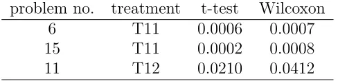
Table 2: Within treatment comparison by problems for T11 and T12

problem no. treatment t-test Wilcoxon 6 T11 0.0006 0.0007 15 T11 0.0002 0.0008 11 T12 0.0210 0.0412

Entries are two-tailed p-values

Signs of inconsistency at the level of problems within treatments were thus fairly weak. We now analyze consistency across the two treatments, by studying whether difference in allocation varies between them for any problem.

We found inconsistency only for two problems, nos. 6 and 15 identified in the prior table. Table 3 below gives results of comparison tests for these two. All tests gave consistency for all other problems.

Table 3: Accross treatment comparisons by problems problem no. t-test Mann-Whitney

6 0.0200 0.0180 15 0.0002 0.0011

Entries are two-tailed p-values

There was thus no inconsistency for at least 90% of the problems in either treatment. Further, different problems showed inconsistency in the two treatments, yielding no par-ticular pattern.5

Our overall conclusion therefore is that the signs of consistency found in the aggregate are strongly supported at the level of individual problems.

3.1.2 Subjects

We now perform disaggregation at the level of subjects. Since every subject participated in only one treatment, this analysis is within treatment only. The question is whether any of these 70 subjects in the two treatments individually displayed inconsistency. We can use choice data from the 20 reference problems faced by any subject to help us address

4

The numbers of the problems in the table refer to an order independent of the ones implemented in the treatments.

5

this matter. We pursued two approaches, one based on comparison tests, and the other on regression.

For the former, we compared the first and second occasion allocations for every subject, using Wilcoxon tests and matched sample t-tests. A subject’s choices were deemed to be inconsistent if a significant difference was found between allocations from the two occasions.

We used a Newey-West adjusted OLS, to account for possible failure of independence at the level of the individual subject arising from some correlation in observation errors across time, for the latter. Specified lags of 0, 1 and 2 yielded similar results, and we only report outcomes for lag 1.

For any regression our specification used the difference in allocation across the two occasions as dependent variable. No independent variable was specified. A constant was used. Thus significance of the constant provides support to the hypothesis of inconsistency, as, had choices been consistent, we would have expected the difference to be zero.

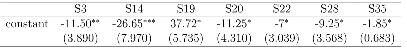
The constant was found to be significant for 7 subjects in T11. Results are shown in Table 4 below.

Table 4: Newey-West regression results for T11

S3 S14 S19 S20 S22 S28 S35

constant -11.50∗∗ _-26.65∗∗∗ _37.72∗ _-11.25∗ _-7∗ _-9.25∗ _-1.85∗

(3.890) (7.970) (5.735) (4.310) (3.039) (3.568) (0.683)

Standard errors in parentheses

∗_{p <0.05,} ∗∗ _{p <0.01,}∗∗∗ _{p <0.001}

For T12, the number of subjects displaying inconsistency was 4. Results are shown in Table 5 below.

Table 5: Newey-West regression resutls for T12 S15 S23 S32 S34 constant 20∗ _15.9∗∗ _-16∗∗∗ _-19.05∗

(9.402) (5.135) (2.706) (7.928)

Standard errors in parentheses

∗ _{p <0.05,}∗∗ _{p <0.01,}∗∗∗ _{p <0.001}

and 4 of the subjects identified in T11. For the remainder, S3, S14 and S19, there was some reduction in significance for S3 and S14, and considerable increase in significance for S19.

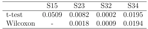
Table 6: t-test and Wilcoxon test resutls for T11

S3 S14 S19 S20 S22 S28 S35 t-test 0.0294 0.0094 0 0.0420 0.0352 0.0327 0.0313 Wilcoxon 0.0246 0.0144 0.0001 - - 0.0177 0.0147

Entries are two-tailed p-values.

Table 7: t-test and Wilcoxon test results for T12 S15 S23 S32 S34 t-test 0.0509 0.0082 0.0002 0.0195 Wilcoxon - 0.0018 0.0009 0.0194

Entries are two-tailed p-values.

Wilcoxon tests showed results which were also similar, but not so close (again, see Tables 6 and 7). For either treatment, a strict subset of the subjects from the regression analysis above were identified to be inconsistent. The absence of S20 and S22 from T11, and S15 from T12 left the number of inconsistent subjects at 5 in T11 and 3 in T12. The levels of significance were also very close for those remaining in T12. The same was found for S28 and S35 in T11, with significant changes for S3, S14 and S19, in the same directions as for the t-tests.

Thus around 10-20% of subjects in total displayed choice inconsistency. With at least 80% of subjects choosing consistently, we conclude overall therefore that the consistency found in the aggregate sample is quite robustly replicated at the level of individual sub-jects.6

Results from Experiment 1 therefore lend considerable support to Hypothesis E. Some support is also given to Hypothesis I (mainly vide findings from Wilcoxon tests reported in Table 1). No evidence is found however to support Hypothesis P.

6

3.2

Experiment 2

The central question remains whether a subject chooses differently the two occasions she faces any reference problem. The measure of consistency in this experiment is the switch rate. For any subject in any treatment, data on two choices are available for any reference problem, one from each occasion it is faced. We will say there is no switch if the two choices made are the same, and there is a switch if the two are different. The switch rate for a subject is then the proportion of times she switched out of 20.

The definition of the switch rate therefore ignores whether the switch was from one definite option to another, or whether it involved indifference (a switch from a definite option to indifference or the other way round).7

As it happens, subjects chose one of the two definite options for an overwhelming majority of problems. The indifference rate (the number of times indifference was reported as a fraction of the total number of problems faced by all subjects taken together) for reference problems was 111/1400 or about 8% for T21 and 152/1400 or about 11% for T22. Additionally, most switches were from one definite option to another: about 70% of all switches in T21 (180/249) and 60% in T22 (54/90).

As indicated in the final sentence of the paragraph above, the aggregate switch rate is 249/700 or 35.5% in T21, and 90/700 or 12.9% in T22. We first test if these are respectively positive. We calculated the switch rate for every subject using the procedure above and tested whether the mean of this sample of 35 observations (using a t-test) for any treatment was different from zero. We found they were: the right-tailed p-values for both treatments were less than 0.001. The same result obtained when we used the median instead of the mean (vide a Snedecor-Cochran sign test).

We then tested if the switch rate was different across the two treatments. The figures given above suggest that the switch rate is higher for T21, where single-contingency situations were faced first relative to T22, where two-contingency situations were faced first. Statistical analysis revealed that average switch rates were indeed different across the two. We performed a t-test as well as a Mann-Whitney test, both of which indicated difference with two-tailed p-values less than 0.001.

Thus the data support the hypothesis that inconsistency may be greater when

single-7

contingency situations are faced earlier in the sequence, so decisions may be more likely to be changed when irrelevant information arrives than when it departs. At the same time, our finding is also that there is significant inconsistency when single-contingency situations are faced later in the sequence. Hence the presence of some inconsistency in decision-making may be endemic, and decisions may be likely to change whenever there is alteration in associated irrelevant information.

We now disaggregate the data, to explore consistency at the levels of the subjects and the problems.

3.2.1 Problems

Within any treatment, every reference problem was faced twice by any subject, and we know for every problem whether a switch occurred or not. Coding a switch as 1, and a consistent choice as 0, we therefore have a series of 35 independent observations (consisting of zeros and ones) for every problem within each treatment.

We tested if the switch rates associated with the problems were positive. We used a t-test as well as a Snedecor-Cochran test for every problem within the two treatments separately. We found severe signs of inconsistency (allowing significance level upto 5%): the null of zero switch rate was rejected for every problem in at least one treatment. Consistency was found for only three problems in T21 (1,3,12) and 6 problems in T22 (6,7,9,14,15,20).8

Tables 8 & 9 below (for T21 and T22 respectively) report right-tailed p-values from the tests, only for the problems displaying inconsistency.

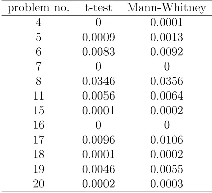
We now analyze consistency across the two treatments for each problem by examining whether there is variation in the switch rate. We found consistency, i.e., statistical indis-tinguishability of switch rates, for 8 problems. Results from these tests are given Table 10 below, which reports two-tailed p-values only for the problems with cross-treatment inconsistency.

There was thus substantive inconsistency within and across treatments for most prob-lems. This leads us to conclude that the inconsistency found in the aggregate is strongly reproduced at the level of individual problems. However the specific pattern found in the aggregate was not replicated, as we found that the inconsistency rate (number of inconsistent problems) did not differ across the treatments, in terms of either a two-tailed or a one-tailed proportion test. The categorization of problems as either consistent or

8

Table 8: t-test and Snedecor-Cochran test resutls for T21 by problems problem no. t-test Snedecor-Cochran

2 0.0016 0.0039

4 0 0

5 0 0

6 0 0.0002

7 0 0

8 0 0

9 0.0060 0.0156 10 0.0003 0.0009

11 0 0

13 0.0032 0.0047 14 0.0016 0.0039

15 0 0

16 0 0

17 0 0.0001

18 0 0

19 0 0

20 0.0001 0.0004

Table 9: t-test and Snedecor-Cochran test resutls for T22 by problems

Table 10: Accross treatments comparison by problems problem no. t-test Mann-Whitney

4 0 0.0001

5 0.0009 0.0013 6 0.0083 0.0092

7 0 0

8 0.0346 0.0356 11 0.0056 0.0064 15 0.0001 0.0002

16 0 0

17 0.0096 0.0106 18 0.0001 0.0002 19 0.0046 0.0055 20 0.0002 0.0003

inconsistent was on the basis of Tables 8 and 9.

3.2.2 Subjects

We now perform disaggregation at the level of subjects. The question is again whether any of these 70 subjects in any treatment individually displayed inconsistency. As before, this is a within treatment analysis.

For every subject, we know whether she switched or not for each of the 20 problems. Consistency would be displayed for a problem by a subject if there is no switch and by the subject overall if the switch rate is zero. We investigate consistency for each subject once again both through comparison tests (t-tests and Snedecor-Cochran tests) as well as through regression analyses.

For the latter approach, we estimated a linear probability model with Newey-West correction for each subject. The strategy mirrors that applied to the data from Experiment 1. The dependent variable indicated whether a switch had been observed or not. There was a constant, but no independent variable. The significance or lack thereof of the constant is used to determine inconsistency or consistency respectively. Lags of 0, 1 and 2 again yielded similar results, and we report only results where lag 1 was specified.

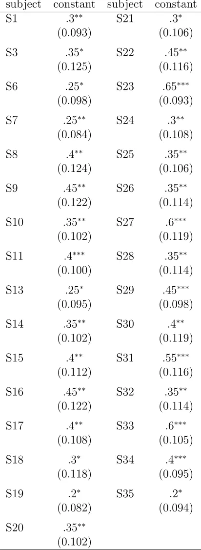
The constant was found to be significant for 31 subjects in T21 (choices of S2, S4, S5 and S12 displayed consistency). Results are shown in Table 11 below in a transposed format.

Table 11: Newey-West regression resutls for T21 subject constant subject constant S1 .3∗∗ _{S21 .3}∗

(0.093) (0.106)

S3 .35∗ _{S22 .45}∗∗

(0.125) (0.116)

S6 .25∗ _{S23 .65}∗∗∗

(0.098) (0.093)

S7 .25∗∗ _{S24 .3}∗∗

(0.084) (0.108)

S8 .4∗∗ _{S25 .35}∗∗

(0.124) (0.106)

S9 .45∗∗ _{S26 .35}∗∗

(0.122) (0.114)

S10 .35∗∗ _{S27 .6}∗∗∗

(0.102) (0.119)

S11 .4∗∗∗ _{S28 .35}∗∗

(0.100) (0.114)

S13 .25∗ _{S29 .45}∗∗∗

(0.095) (0.098)

S14 .35∗∗ _{S30 .4}∗∗

(0.102) (0.119)

S15 .4∗∗ _{S31 .55}∗∗∗

(0.112) (0.116)

S16 .45∗∗ _{S32 .35}∗∗

(0.122) (0.114)

S17 .4∗∗ _{S33 .6}∗∗∗

(0.108) (0.105)

S18 .3∗ _{S34 .4}∗∗∗

(0.118) (0.095)

S19 .2∗ _{S35 .2}∗

(0.082) (0.094)

S20 .35∗∗

(0.102)

Standard errors in parentheses

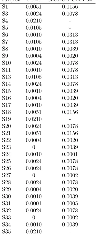
Table 12: t-test and Snedecor-Cochran test resutls for T21 subject t-test Snedecor-Cochran

S1 0.0051 0.0156 S3 0.0024 0.0078

S4 0.0210

-S5 0.0105

-S6 0.0010 0.0313 S7 0.0105 0.0313 S8 0.0010 0.0039 S9 0.0004 0.0020 S10 0.0024 0.0078 S11 0.0010 0.0078 S13 0.0105 0.0313 S14 0.0024 0.0078 S15 0.0010 0.0039 S16 0.0004 0.0020 S17 0.0010 0.0039 S18 0.0051 0.0156

S19 0.0210

-S20 0.0024 0.0078 S21 0.0051 0.0156 S22 0.0004 0.0020

S23 0 0.0039

S24 0.0010 0.0001 S25 0.0024 0.0078 S26 0.0024 0.0078

S27 0 0.0002

S28 0.0024 0.0078 S29 0.0004 0.0020 S30 0.0010 0.0039 S31 0.0001 0.0005 S32 0.0024 0.0078

S33 0 0.0002

S34 0.0010 0.0039

S35 0.0210

p-values as entries. The t-tests find 33 subjects to be inconsistent (all but S2 and S12). The Snedecor-Cochran procedure yields the number 29 (all but S2, S4, S5, S12, S19 and S35).

For T22, the number of subjects displaying inconsistency was 7 (S3, S8, S14, S15, S16, S24 and S35), according to the regression approach. Results are shown in Table 13 below.

Table 13: Newey-West regression reults for T22

S3 S8 S14 S15 S16 S24 S35

constant -.45∗∗∗ _.25∗∗ _.2∗ _.35∗∗ _.2∗ _.25∗∗ _.45∗∗∗

(0.091) (0.084) (0.082) (0.106) (0.094) (0.084) (0.091)

Standard errors in parentheses

∗ _{p <0.05,}∗∗ _{p <0.01,}∗∗∗ _{p <0.001}

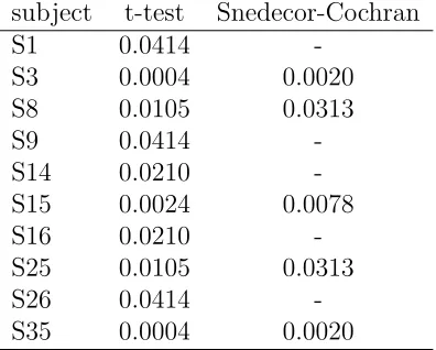
Comparison tests yielded somewhat similar results for T22. The results are shown in Table 14 (entries are right-tailed p-values). The t-tests determined 10 subjects to be inconsistent (S1, S3, S8, S9, S14, S15, S16, S25, S26 and S35) while the Snedecor-Cochran tests found 5 (S3, S8, S15, S25 and S26).

Table 14: t-test and Snedecor-Cochran test resutls for T22 subject t-test Snedecor-Cochran

S1 0.0414

-S3 0.0004 0.0020 S8 0.0105 0.0313

S9 0.0414

-S14 0.0210

-S15 0.0024 0.0078

S16 0.0210

-S25 0.0105 0.0313

S26 0.0414

-S35 0.0004 0.0020

Entries are right-tailed p-values

is replicated at the level of individual subjects. Moreover, the pattern was also similar to that in the aggregate: a proportion test of whether the inconsistency rate (number of inconsistent subjects) differed across the treatments showed that the rate was higher in T21 (p-value <0.001). Categorization of subjects as either consistent or inconsistent was done on the basis of Tables 11 and 13.

Results from Experiment 2 therefore unambiguously support Hypothesis P. No evi-dence is found in favor Hypotheses I or E.

4

Conclusions

This paper reports results from experiments examining whether subjects’ contingent choices satisfy consistency. It found that consistency may mostly be a reasonable pre-sumption when contingencies are complete, and outcomes are monetary and immediate, but is unlikely to fully hold in more complex and realistic settings.

We further found that decisions may be more likely to change when irrelevant or extraneous information arises rather than subsides. Since actual decisions are often one-shot and made in the presence of both irrelevant and relevant information, this suggests that experimental explorations of consistency using a within subject design should control for order effects to improve accuracy of results. Hence studies which only expose subjects first to relevant information, and then to all information, relevant as well as irrelevant, without counterbalancing, such as Dror, Charlton and P´eron [3], may be overstating the degree of inconsistency.

References

[1] Bodenhausen, G. and R. Wyer (1985): Effects of Stereotypes on Decision Making and Information-Processing Strategies, Journal of Personality and Social Psychol-ogy, 48, 267-82.

[2] Coman, D., A. Coman and W. Hirst (2013): Memory Accessibility and Medical Decision-Making for Significant Others: the Role of Socially Shared Retrieval-Induced Forgetting, Frontiers in Behavioral Neuroscience, 7, article 72.

[3] Dror, I., D. Charlton and A. P´eron (2006): Contextual Information Renders Ex-perts Vulnerable to Making Erroneous Identifications, Forensic Science Interna-tional, 156, 74-8.

[4] Fabozzi, F., P. Kolm, D. Pachamanova and S. Forcardi (2007): Robust Portfoilio Optimization and Management. Wiley: Hoboken, New Jersey.

[5] Green, E. and K. Osband (1991): Revealed Preference Theory for Expected Utility,

Review of Economic Studies, 58, 677-95.

[6] Green, E. and I. Park (1996): Bayes Contingent Plans, Journal of Economic Be-havior & Organization, 31, 225-36.

[7] Heston, A., R. Summers and B. Aten (2012): Penn World Table Version 7.1, Cen-ter for InCen-ternational Comparisons of Production, Income and Prices, University of Pennsylvania.

[8] Jones, M. and B. Love (2011): Bayesian Fundamentalism or Enlightenment? On the Explanatory Status and Theoretical Contributions of Bayesian Models of Cognition,

Behavioral and Brain Sciences, 34, 169-231.

[9] Jørgensen, M. and S. Grimstad (2011): The Impact of Irrelevant and Misleading Information on Software Development Effort Estimates: A Randomized Controlled Field Experiment, IEEE Transactions on Software Engineering, 37, 695-707.

[10] Rubinstein, A. (2012): Lecture Notes in Microeconomic Theory, 2nd edition. Prince-ton: Princeton University Press.

[12] Savage, L. (1972): The Foundations of Statistics, 2nd edition. New York: Dover.

[13] Zambrano, E. (2005): Testable Implications of Subjective Expected Utility Theory,

Games and Economic Behavior, 53, 262-68.

Appendix

Instructions for Experiment 1:

Thank you for your participation. Please read the instructions carefully.

You will face 40 questions one after the other. After finishing a question, please press the CONTINUE button, and the next question will appear.

Here is a sample question:

You have decided to invest 100 rupees by buying units of financial options. There are two options available, and one unit costs 1 rupee for either option. The table below gives the possible returns and the corresponding chances per unit for both. How much of your 100 rupees will you invest in option 1, i.e., how many units of option 1 will you buy? Whatever remains will be used to buy units of option 2. Your answer must be an integer between and including 0 and 100.

O1 O2

return chance return chance

2.2 0.2 3.1 0.4 0.9 0.8 0.6 0.6

Thus, your answer here will be the number of units of option 1 you are buying. Here is another sample question:

You have decided to invest 100 rupees by buying units of financial options. There are two options available, and one unit costs 1 rupee for either option. The table below gives the possible returns and the corresponding chances per unit for both. How much of your 100 rupees will you invest in option 1, i.e., how many units of option 1 will you buy? Whatever remains will be used to buy units of option 2. Your answer must be an integer between and including 0 and 100.

O1 O2 return chance return chance

2.2 0.2 3.1 0.4 0.9 0.8 0.6 0.6

What if the options are instead (again, what you do not invest in 1A

will be automatically invested in 2A and your answer must be an integer):

O1A O2A

return chance return chance

2.5 0.25 4 0.5

0.1 0.75 0.7 0.5

For every question, you will have to allocate 100 across two options each with two possible returns. Here is an example on what you might expect to get as return, using the second sample question.

Suppose you have chosen to invest 70 in option 1 and therefore 30 in option 2 for the first case, and for the second case your choice is 40 in option 1A and therefore 60 in option 2A.

Then the outcomes for the first case can be either:

(1) 2.2 in option 1, and 3.1 in option 2. The chance of this is 0.2∗ ×0.4 = 8%.Then your return is 70×2.2 + 30×3.1 = 247

(2) 2.2 in option 1, and 0.6 in option 2. The chance of this is 0.2×0.6 = 12%. Then your return is 70×2.2 + 30×0.6 = 172

(3) 0.9 in option 1, and 3.1 in option 2. The chance of this is 0.8×0.4 = 32%. Then your return is 70×0.9 + 30×3.1 = 156

(4) 0.9 in option 1, and 0.6 in option 2. The chance of this is 0.8×0.6 = 48%. Then your return is 70×0.9 + 30×0.6 = 81

And the outcomes for the second case can be either:

(2) 2.5 in option 1, and 0.7 in option 2. The chance of this is 0.25×0.5 = 12.5%. Then your return is 40×2.5 + 60×0.7 = 142

(3) 0.1 in option 1, and 4 in option 2. The chance of this is 0.75×0.5 = 37.5%. Then your return is 40×0.1 + 60×4 = 244

(4) 0.1 in option 1, and 0.7 in option 2. The chance of this is 0.75×0.5 = 37.5%. Then your return is 40×0.1 + 60×0.7 = 46

As you know, you will earn money for today’s participation, and how much you will earn will depend on how you decide and some luck. Five of your investment choices will be picked at random at the end, and their corresponding options will be implemented in accordance with your choices. You will get the average of their returns, plus a fee for showing up.

Let’s start! Read the questions carefully, and then choose.

Instructions for Experiment 2:

Thank you for your participation. Please read the instructions carefully.

You will face 40 questions one after the other. Here is a sample question:

You have to choose one of the three options - C1, C2, C3. Put a tick (X_{) in the}

relevant box.

Which cup would you prefer if the options are C1, C2 and C3?

C1 _{C2 C3}

1. Small 1. Small-Medium 2. No handle. 2. With handle

3. White with floral pattern 3. Light yellow no pattern Indifferent 4. Normal design 4. Octagonal design.

Please choose only one out of the three options. You are thus giving a single answer here.

Here is another sample question:

Which cup would you prefer if the options are C1, C2 and C3?

C1 _{C2 C3}

1. Small 1. Small-Medium 2. No handle. 2. With handle

3. White with floral pattern 3. Light yellow no pattern Indifferent 4. Normal design 4. Octagonal design.

What if the options are instead

C1A _{C2A C3A}

1. Small-Medium 1. Small

2. Base smaller than rim. 2. Base and rim are of same size

3. Black with geometric pattern 3. White with blue band Indifferent 4. Hexagonal design 4. Hexagonal design.

For every question, you will face some good, durable, activity, asset or service, with four characteristics given for any option. There will be two main options. You will have to compare and choose one of them. Or you can be indifferent.