Native Language Identification With Classifier Stacking and Ensembles

Classifier Stacking and Ensembles

Shervin Malmasi

Mark Dras

Macquarie University Department of Computing [email protected]

Ensemble methods using multiple classifiers have proven to be among the most successful approaches for the task of Native Language Identification (NLI), achieving the current state of the art. However, a systematic examination of ensemble methods for NLI has yet to be conducted. Additionally, deeper ensemble architectures such as classifier stacking have not been closely evaluated. We present a set of experiments using three ensemble-based models, testing each with multiple configurations and algorithms. This includes a rigorous application of meta-classification models for NLI, achieving state-of-the-art results on several large data sets, evaluated in both intra-corpus and cross-corpus modes.

1. Introduction

Native Language Identification (NLI) is the task of identifying a writer’s native lan-guage (L1) based only on their writings in a second lanlan-guage (the L2). NLI works by identifying language use patterns that are common to groups of speakers of the same native language. This process is underpinned by the presupposition that an author’s L1 disposes them towards certain language production patterns in their L2, as influenced by their mother tongue. This relates to cross-linguistic influence, a key topic in the field of Second Language Acquisition (SLA), which analyzes transfer effects from the L1 on later learned languages (Ortega 2009).

It has been noted in the linguistics literature since the 1950s that speakers of par-ticular languages have characteristic production patterns when writing in a second language. This language transfer phenomenon has been investigated independently in various fields from different perspectives, including qualitative research in SLA and recently via predictive models in NLP (Jarvis and Crossley 2012). Recently, this has motivated studies in NLI, a subtype of text classification where the goal is to determine the native language of an author, using texts that they have written in a second language (Tetreault, Blanchard, and Cahill 2013).

Submission received: 18 October 2016; Revised version received: 1 August 2017; Accepted for publication: 6 April 2018.

doi:10.1162/COLI a 00323

© 2018 Association for Computational Linguistics

The motivations for NLI are manifold. Such techniques can help SLA researchers identify important L1-specific learning and teaching issues. In turn, the identification of such issues can enable researchers to develop pedagogical material that takes into con-sideration a learner’s L1 and addresses them. It can also be applied in a forensic context, for example, to glean information about the discriminant L1 cues in an anonymous text. NLI is most commonly framed as a multiclass supervised classification task. Re-searchers have experimented with a range of machine learning algorithms, with support vector machines (SVMs) having found the most success. However, some of the most successful approaches have made use of classifier ensemble methods to further improve performance on this task. This is a trend that has become apparent in recent work on this task, as we will outline in Section 2. In fact, all recent state-of-the-art systems have relied on some form of multiple classifier system.

However, a thorough examination of ensemble methods for NLI—one empirically comparing different architectures and algorithms—has yet to be conducted. Addition-ally, more sophisticated ensemble architectures, such as classifier stacking, have not been closely evaluated. This meta-classification approach is an advanced method that has proven to be effective in many classification tasks; its systematic application could improve the state of the art in NLI.

This has links to the idea of adding layers to increase power in neural network– based deep learning, which has come to be an important approach in NLP over the last few years (Manning 2015); Eldan and Shamir (2016, page 907) note that “Overwhelming empirical evidence as well as intuition indicates that having depth in the neural network is indeed important.” Deep neural networks can in fact be seen as layered classifiers (Goldberg 2015), and ensemble methods as an alternative way of adding power via additional layers. In this article we look just at ensemble methods: Deep learning has not yet produced state-of-the-art results on related tasks (Malmasi et al. 2016),1_{and our} goal is to understand what it is that has made ensemble methods to date in NLI so successful.

The primary focus of the present work is to address this gap by presenting a com-prehensive and rigorous examination of how ensemble methods can be applied for NLI. We aim to examine several different ensemble and meta-classification architectures, each of which can utilize different configurations and algorithms.

Furthermore, previous ensemble methods have not been tested on different data sets, making the ability of these models to generalize for NLI unclear. Ideally, the same method should be tested across multiple corpora to assess its validity. To this end, we also apply our methods to multiple data sets, in both English and other languages, to evaluate their generalization capacity. In addition, following the observation of Brooke and Hirst (2012b) that patterns utilized by machine learners can be corpus-specific and influenced by topic, even with apparently topic-neutral features—something that could also be true in our multi-level classifier context—we carry out cross-corpus experiments along the lines of Brooke and Hirst (2012b), Malmasi and Dras (2015), and Ionescu, Popescu, and Cahill (2016).

To summarize, the principal aims of the present study are the following:

1. Apply several advanced ensemble combination methods to NLI and evaluate their performance against previously used ensemble methods.

1 Traditional text classification methods substantially outperformed all deep learning approaches in the 2016 DSL Shared Task.

2. Evaluate the use of meta-classifiers for NLI, applying different feature representations and a range of learning algorithms.

3. Compare the performance of these methods with previous results and assess the methods on, and between, different data sets.

The remainder of this paper is organized as follows. In Section 2 we introduce ensemble classification and recap previous work in NLI. Our data are introduced in Section 3, followed by our experimental set-up in Section 4, and our classification fea-tures in Section 5. Our ensemble-based models are detailed in Section 6 and experimen-tal results are reported in Section 7. We then conclude with a discussion in Section 8.

2. Related Work

This work draws on two broad areas of research: ensemble-based classification methods and work in NLI.

2.1 Ensemble Classifiers

Classifier ensembles are a way of combining different classifiers or experts with the goal of improving overall accuracy through enhanced decision making. Instead of relying on decisions by a single expert, they attempt to reach a decision by utilizing the collective input from a committee of experts.

They have been applied to a wide range of real-world problems and have been shown to achieve better results compared with single-classifier methods (Oza and Tumer 2008). Through aggregating the outputs of multiple classifiers in some way, their outputs are generally considered to be more robust. Ensemble methods continue to receive increasing attention from investigators and remain a focus of machine learning research (Kuncheva and Rodr´ıguez 2014; Wo´zniak, Gra ˜na, and Corchado 2014).

Such ensemble-based systems often use a parallel architecture, where the classifiers are run independently and their outputs are aggregated using a fusion method. The specifics of how such systems work will be detailed in Section 6.

They have been applied to various classification tasks with good results. Not sur-prisingly, researchers have attempted to use them for improving the performance of NLI, as we discuss in the next section.

2.2 Native Language Identification

General Background.Determining the identity of, or properties of, an author of a text is a problem of longstanding interest, and attempts to solve it are similarly longstand-ing (Koppel, Schler, and Argamon 2009). NLI is the subtype of this task focuslongstand-ing on identifying the L1 of the writer. To our knowledge, the first work tackling this task in a computational manner was that of Tomokiyo and Jones (2001), who worked with speech data recorded for this task. Their main aim was to detect non-native speech, using part-of-speech and lexical features in a na¨ıve Bayes classifier, and to also deter-mine the native language of the non-native speakers. Another early work was that of Jarvis, Castaneda-Jim´enez, and Nielsen (2004), who presented an early empirical approach to investigating L1 transfer using lexical style and word choice, which they termedwordprints. Working with a written corpus compiled for the task and focusing exclusively on lexical transfer, they collected the 30 most frequent words used by each

group of L1 speakers, resulting in a set of 53 words that were used as features in a Linear Discriminant Analysis (LDA) classifier.

The framework that is now most commonly used for NLI was introduced by Koppel, Schler, and Zigdon (2005b). They used essay-style texts drawn from the In-ternational Corpus of Learner English (Granger et al. 2009), and a similar multiclass classification paradigm to the earlier work, with an SVM classifier. Their features were broader than the earlier work, and included syntactic, lexical, and stylistic features, such as function words (e.g., and,from, which,whilst), charactern-grams (i.e.,sequences of characters of lengthn), and PoS bi-grams, together with some spelling mistakes.

The volume of work then built from further investigation by Wong and Dras (2009). A detailed review of NLI methods is omitted here for reasons of space, but a thorough exposition of work predominantly carried out within the NLP community within the framework set out by Koppel, Schler, and Zigdon (2005a) is presented in the report from the first NLI Shared Task2_{that was held in 2013 (Tetreault, Blanchard, and Cahill 2013).} Jarvis and Crossley (2012) present a collection of work from the SLA community, all using LDA classification and features that include wordn-grams, lexical and semantic indices, and error categories.

Most English NLI work has been done using two corpora. The above-mentioned International Corpus of Learner English (Granger et al. 2009) was widely used until recently, despite its shortcomings3 being widely noted (Brooke and Hirst 2012a). More recently, TOEFL11, the first corpus designed for NLI, was released (Blanchard et al. 2013). Although it is the largest NLI data set publicly available, it only contains argumentative essays, limiting analyses to this genre. Research has also expanded to use non-English learner corpora (Malmasi and Dras 2014a,c).

Ensemble Methods: The 2013 Shared Task.As mentioned earlier, some of the most success-ful approaches to NLI have used ensemble learning methods, and investigating ensem-ble configurations is a key goal of this article. We now therefore present an overview of work in NLI that has used ensembles, focusing on the way in which ensembles were defined and what benefit they brought. Most of this work leads into, is part of, or is positioned with respect to the first NLI shared task of 2013. We discuss briefly after this some observations from the 2017 shared task.

Tetreault et al. (2012) were the first to propose the use of classifier ensembles for NLI, and they performed a comprehensive evaluation of the feature types used until that point. In their study they used an ensemble of logistic regression learners, using a wide range of features that included character and wordn-grams, function words, parts of speech, spelling errors, and writing quality markers. With regard to syntactic features, they also investigated the use of Tree Substitution Grammars and dependency features extracted using the Stanford parser. Furthermore, they also proposed using language models for this task and in their system used language model perplexity scores based on lexical 5-grams from each language in the corpus. The set of features used here was the largest of any NLI study to date. With this system, the authors reported state-of-the-art accuracies with the ensemble model of 90.1% and 80.9% on the ICLE and TOEFL11 corpora, respectively. The ensemble model improved over a simple concatenation of all feature vectors by 7.5% and 4.9% on the respective corpora. Tetreault et al. also conducted cross-corpus evaluation, using the seven common L1 classes between the

2https://sites.google.com/site/nlisharedtask2013/home. 3 The issues exist as the corpus was not designed specifically for NLI.

ICLE and TOEFL11 corpora. Training on the ICLE data, they report an accuracy of 26.6%.

The subsequent 2013 NLI Shared Task, attracting entries from 29 teams, saw many approaches that used ensembles.

The winning entry for the shared task did not use an ensemble, but we summarize it to put the other work into context. This system, by Jarvis, Bestgen, and Pepper (2013), had an accuracy of 83.6%, using as featuresn-grams of words, parts-of-speech, as well as lemmas. In addition to normalizing each text to unit length, the authors also applied a log-entropy weighting schema to the normalized values, which clearly improved the accuracy of the model. An L2-regularized SVM classifier was used to create a single-model system. Furthermore, the authors used their own procedure for optimizing the cost parameter (C) of the SVM. Although they did not use a great number of features or introduce any new features for this task, and they did not use an ensemble, we posit that their use of weighting schema and hyperparameter optimization gave their system an edge over their competitors, the majority of whom did not utilize these techniques.

Gyawali, Ramirez, and Solorio (2013) utilized lexical and syntactic features based onn-grams of characters, words, and part-of-speech tags (using both the Penn Tree-Bank and Universal Parts Of Speech tagsets), along with perplexity values of character n-grams to build four different models. These models were combined using a voting-based ensemble of SVM classifiers. Features values were weighted using the TF-IDF scheme. In particular, the authors set out to investigate whether a more coarse-grained POS tagset would be useful for NLI. They explored the use of the Universal POS tagset, which has 12 POS categories in the NLI shared task, and compared the results with the fine-grained Penn Treebank (PTB) tagset, which includes 36 POS categories. The highest accuracy of their system in the shared task was 74.8%, achieved by combining all fea-tures into an ensemble. The authors found that the use of coarse-grained Universal POS tags as features generalizes the syntactic information and reduces the discriminative power of the feature that comes from the fine granularity of then-grams. For example, the PTB tagset distinguishes verbs into six distinct categories, whereas the Universal POS tagset only has a single category for that grammatical class.

In the system designed by Cimino et al. (2013), the authors used a wide set of general-purpose features, designed to be portable across languages, domains, and tasks. This set included features that are lexical (sentence length, document length, type/token ration, character and wordn-grams), morpho-syntactic (coarse and fine-grained part-of-speech tagn-grams), and syntactic (parse tree and dependency-based features). They found distributional differences across the L1s for many of these features, including average word and sentence lengths. However, we note that many of these differences are not of a large magnitude, and the authors did not run any statistical tests to measure the significance levels of these differences. Using this feature set, they experimented with a single-classifier system as well as classifier ensembles, using SVM and Maxi-mum Entropy classifiers. In their ensemble, they experimented with using a majority voting system as well as a meta-classifier approach. The authors reported that the ensemble methods outperformed all single-classifier systems (by around 2%), and their best performance of 77.9% was provided by the meta-classifier system that used linear SVM and MaxEnt as the component classifiers and combined the results using a poly-nomial kernel SVM classifier. Although the set of features used in this experiment is not widely different from other reported NLI research, their use of a meta-classifier is an interesting approach that warrants further study.

In their system, Goutte, L´eger, and Carpuat (2013) used character, word, and part-of-speech n-grams, along with syntactic dependencies. They used an ensemble of

SVM classifiers trained on each feature space, using a majority vote combiner method. To represent the feature values, they used two value normalization methods based on TF-IDF and cosine normalization. Their best entry achieved an accuracy of 81.8%, higher than many systems using the same standard features and more, demonstrating the effec-tiveness of using ensemble classifiers and appropriate feature value representation. The authors, like many others, also noted that lexical features provided the best performance for a single feature in their system, but that this can be boosted by combining multiple predictors.

The MITRE system (Henderson et al. 2013) was another highly lexicalized system where the primary features used are word, part-of-speech, and character n-grams. In this system, these features are used by independent classifiers (logistic regression, Winnow2, and language models) whose output is then combined into a final prediction, using a na¨ıve Bayes model. Their best performing ensemble was 82.6% accurate in the shared task and the authors emphasized the value of ensemble methods that combine independent systems. Furthermore, the authors also optimized the parameters of their na¨ıve Bayes model using a grid search over the development data.

Hladka, Holub, and Kriz (2013) developed an ensemble classifier system, using some standard features (lemma, word, and part-of-speechn-grams, word skipgrams) with SVM classifiers. They obtained an accuracy of 72.5% in the shared task. They found that their ensemble, which was based on majority voting, outperformed other methods of combining the features.

Another system that utilized an ensemble is that of Bykh et al. (2013), where they used a probability-based ensemble. They used a set of 16 features, including recurring word-basedn-grams, recurring Open Class POSn-grams, dependencies, trees, and lem-mas. To combine the different feature types, they explored combining all features into a single vector and also ensembles of SVM classifiers (each trained on a single feature type). Their best shared task performance of 82.2% was achieved using an ensemble with all of their features; among these features, recurring word-basedn-grams are the best performing single feature type.

Following the shared task, Bykh and Meurers (2014) further explored the use of lexicalized and non-lexicalized phrase structure rules for NLI. They showed that the inclusion of lexicalized production rules (i.e., preterminal nodes and terminals) pro-vides improved results. In addition to the standard normalized frequency and binary feature representations, they also proposed two new representations based on a “vari-ationist sociolinguistic” perspective. Although they showed that these representations outperformed the normalized frequency approach, they did not compare this to other representations that have been shown to improve NLI accuracy, such as TF-IDF. They combined their lexicalized production rules feature with additional surface n-gram features in a tuned and optimized ensemble, reporting an accuracy of 84.82% on the TOEFL11-TESTset.

Ionescu, Popescu, and Cahill (2014) extended the previous work of Popescu and Ionescu (2013), which used string kernels to perform NLI, using only charactern-gram features. One improvement here is that several string kernels are combined through multiple kernel learning. Although this approach is not based on the types of ensembles we use here, it is similar in the sense that it attempts to combine multiple learners. The authors also performed parameter tuning to select the optimal settings for their system. They reported an accuracy of 85.3% on the TOEFL11-TEST set, 1.7% higher than the winning shared task system. Recently, they expanded their approach with additional experiments (Ionescu, Popescu, and Cahill 2016), although they did not achieve further improvements on TOEFL11-TEST.

Ensemble Methods: The 2017 Shared Task.The 2017 NLI shared task saw a similar level of interest as the 2013 one, with 19 teams participating. The framework was broader than for 2013, looking at NLI based on both text and speech, with three tracks in the task: essay-only, speech-only, and fusion. The essay-only track, which we focus on here, was very similar to the 2013 task, and also based on TOEFL essays. This time, the training set consisted of the TOEFL11 training and development sets, the development set was the TOEFL11 test set, and there was a new test set. (Consequently, the accuracies for systems that took part in this task are not directly comparable with those discussed earlier.) Ranking of systems also involved the use of McNemar’s test for statistical significance, which determined five bands of performance that were statistically indistinguishable.

Again, several systems used classifier stacking or ensembles of classifiers, including the top system, and we discuss these briefly. The 2017 shared task took place after the release of the first version of this paper,4_{and the systems that used classifier ensembles} or stacking for the most part cited this work as the source of the architectural framework used. In the top band of seven systems (accuracies 86.5% to 88.2%), three of the best systems from each team (Cimino and Dell’Orletta 2017; Goutte and L´eger 2017; Li and Zou 2017) used the architectures described later in this paper, with the same kinds of base machine learners, but incorporating some variations: for instance, Cimino and Dell’Orletta (2017) additionally used a sentence-level classifier. In the second band of three systems (accuracies 85.4% to 86.4%), all used ensembles (Chan et al. 2017; Ircing et al. 2017; Oh et al. 2017). Interestingly, this band included the highest-ranked system to incorporate deep learning (Oh et al. 2017), supporting our earlier observation that a state-of-the-art deep learning architecture for this kind of classification task has not yet been identified. Two systems that explored deep learning architectures (Bjerva et al. 2017; Sari, Rifqi Fatchurrahman, and Dwiastuti 2017) were ranked in the third band.

One new observation that can be made from the systems in this 2017 task is that although some systems found that more features can be helpful (Cimino and Dell’Orletta 2017; Goutte and L´eger 2017; Li and Zou 2017; Markov et al. 2017), some found that fewer were better (Ionescu and Popescu 2017; Kulmizev et al. 2017; Rama and C¸ ¨oltekin 2017).5 _{In one case (Rama and C¸ ¨oltekin 2017) this was specific to the} fusion task, rather than the essay task, but in one other (Kulmizev et al. 2017) a single SVM with only charactern-grams performed better than some ensemble architectures motivated by the previous version of the present paper (Malmasi and Dras 2017b). The motivation of a systematic exploration of ensemble architectures that is the goal of the present paper is thus still of broad interest.

In sum, we can see that ensemble-based approaches have yielded some of the most successful results in this field. However, we also believe that it is possible to use ensemble models that are even more sophisticated, leading to improved results. This is the key research question we investigate in the present study.

3. Data

We now introduce the data sets used in this study.

One of the goals of this study is to assess the generalization capability of the methods and results across data sets, so we consequently use two corpora that have been used in previous NLI work.

4 We made this available athttps://arxiv.org/abs/1703.06541, as Malmasi and Dras (2017b). 5 We thank an anonymous reviewer for this observation.

3.1 The TOEFL11 Corpus

The TOEFL11 corpus (Blanchard et al. 2013)—also known as the Educational Testing Service Corpus of Non-Native Written English—is the first data set designed specifically for the task of NLI and developed with the aim of addressing the above-mentioned deficiencies of other previously used corpora. By providing a common set of L1s and evaluation standards, the authors set out to facilitate the direct comparison of approaches and methodologies.

Furthermore, as all of the texts were collected through the Educational Testing Service’s electronic test delivery system, this ensures that all of the data files are encoded and stored in a consistent manner.6_{The corpus is available through the Linguistic Data} Consortium.7

It consists of 12,100 learner texts from speakers of 11 different languages. The texts are independent task essays written in response to eight different prompts, and were collected in the process of administering the Test of English as a Foreign Language (TOEFL) between 2006 and 2007. The texts are divided into specific training (TOEFL 11-TRAIN), development (TOEFL11-DEV), and test (TOEFL11-TEST) sets. It is also com-mon to combine the training and development sets for training, which we refer to as TOEFL11-TRAINDEV.

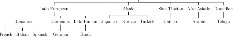
The 11 L1s are Arabic, Chinese, French, German, Hindi, Italian, Japanese, Korean, Spanish, Telugu, and Turkish. This selection ensures that there are L1s from diverse language families, but also several from within certain families. The L1s and their language families are shown in Figure 1.

This data set was designed specifically for NLI and the authors attempted to balance the texts by topic and native language. There are a total of eight essay prompts in the corpus, with the prompts setting each essay’s topic or theme. Although they were not able to create a perfectly balanced corpus, the distribution of topics across L1s is very even.8_{This distribution of essay prompts by L1 is shown in Figure 2.}

3.2 The EFCAMDATCorpus

The EF Cambridge Open Language Database (EFCAMDAT) is an English L2 corpus that was released in 2013 (Geertzen, Alexopoulou, and Korhonen 2013) and used for NLI in Malmasi and Dras (2015).

EFCAMDATis composed of texts submitted toEnglishtown, an online school used by thousands of learners daily. This corpus is a large one, containing some 550k texts from numerous nationalities. Whereas TOEFL11 is made of argumentative essays, EFCAMDAThas a much wider range of genres including writing e-mails, descriptions, letters, reviews, instructions, and more.

Malmasi and Dras (2015) used this corpus for two purposes: to apply NLI to another large-scale corpus for L2 English that differ in the characteristics (e.g., genre) of its constituent texts; and to carry out a large-scale cross-corpus analysis, following earlier

6 The essays are distributed as UTF-8 encoded text files. 7https://catalog.ldc.upenn.edu/LDC2014T06.

8 Kulmizev et al. (2017) observed that this does not perfectly prevent an NLI from improving performance via topic modeling. They replaced the top 100 keywords per prompt in TOEFL11, determined using a sparse additive generative model, with a dummy string, and observed that performance dropped by around 2%. Nevertheless, the even distribution of topics in TOEFL11 does mitigate this to some extent, compared with the earlier ICLE corpus.

Dravidian Telugu Afro-Asiatic Arabic Sino-Tibetan Chinese Altaic Turkish Korean Japanese Indo-European Indo-Iranian Hindi Germanic German Romance Spanish Italian French

Figure 6. Language families in corpus

16 Figure 1

Language families in the TOEFL11 corpus. The languages were selected to represent different families, but to also have several from within the same families. Diagram reproduced from Blanchard et al. (2013) with permission.

0 50 100 150 0 50 100 150 0 50 100 150 0 50 100 150 0 50 100 150 0 50 100 150 0 50 100 150 0 50 100 150 P1 P2 P3 P4 P5 P6 P7 P8

Ara. Chi. Fre. Ger. Hin. Ita. Jap. Kor. Spa. Tel. Tur.

Language Essa ys Language Arabic Chinese French German Hindi Italian Japanese Korean Spanish Telugu Turkish

Figure 2. Number of essays per language per prompt

12 Figure 2

A plot of how the eight topic prompts are distributed across the L1 groups in the TOEFL11 corpus. Prompts are labeled P1–P8. Figure reproduced from Blanchard et al. (2013) with permission.

Table 1

The 11 L1 classes extracted from the EFCAMDATcorpus, compared with the TOEFL11 corpus. The first 9 classes are common to both.

Common Arabic, Chinese, French, German, Italian, Japanese, Korean, Spanish, Turkish EFCAMDAT Portuguese, Russian

TOEFL11 Hindi, Telugu

work by Brooke and Hirst (2012b) and Tetreault et al. (2012) on other, smaller corpora. Brooke and Hirst (2012b, page 392) note that patterns utilized by machine learners can be corpus-specific, and can be influenced by topic, even with apparently topic-neutral features; but that “any variation that is consistent across very distinct corpora is likely to be a true indicator of L1.” Following Malmasi and Dras (2015), we use EFCAMDAT for both within-corpus and cross-corpus evaluations—training on TOEFL11 and testing on EFCAMDAT, and vice versa—and apply the same set-up for our experiments with the data set, which we recap here.

As some of the texts in EFCAMDATcan be short, Malmasi and Dras (2015) followed the methodology of Brooke and Hirst (2011) to concatenate and create texts with at least 300 tokens, producing texts similar in size to TOEFL11. From the data 850 texts were chosen from each of the top 11 nationalities, the same number of L1s as in TOEFL11 to allow a more direct comparison of classifier accuracies (see Table 1 for the languages). This subset of EFCAMDAT thus consists of 9,350 documents totalling approximately 3.2m tokens. This is an average of 337 tokens per text, close to the 348 tokens per text in TOEFL11. The within-corpus experiments use this whole subset, whereas the cross-corpus experiments use just the nine languages in common between EFCAMDAT and TOEFL11. There is no separate test set for this corpus.

3.3 The ASK Corpus

In this study we use data from the ASK Corpus (Andrespr˚akskorpus [Second Lan-guage Corpus]). The ASK Corpus (Tenfjord, Meurer, and Ragnhildstveit 2013; Tenfjord, Johansen, and Hagen 2006; Tenfjord, Meurer, and Hofland 2006) is a learner corpus composed of the writings of learners of Norwegian. These texts are essays written as part of a test of Norwegian as a second language. Each text also includes additional metadata about the author such as age or native language. A positive feature of this corpus is that all the texts have been collected under the same conditions and time limits. The corpus also contains a control subcorpus of texts written by native Norwegians under the same test conditions. The corpus also includes error codes and corrections, although we do not make use of this information here.

There are a total of about 1,700 essays9 _{written by learners of Norwegian as a} second language with ten different first languages: German, Dutch, English, Spanish, Russian, Polish, Bosnian-Croatian-Serbian, Albanian, Vietnamese, and Somali. The essays are written on a number of different topics, but these topics are not balanced across the L1s.

9 Tenfjord, Meurer, and Ragnhildstveit (2013), in the description of the corpus, remark that it consists of 1,700 essays. However, we received 1,736 essays from the corpus maintainers.

Detailed word-level annotations (lemma, POS tag, and grammatical function) have been first obtained automatically, using the Oslo-Bergen tagger. These annotations have then been manually post-edited by human annotators because the tagger’s performance can be substantially degraded due to orthographic, syntactic, and morphological learner errors. These manual corrections can deal with issues such as unknown vocabulary or wrongly disambiguated words.

We use two different derived data sets for Norwegian, which we term “raw” and “generated.”

Raw Data Set.This consists of just the full set of original documents.

Generated Data Set.Unlike TOEFL11, the ASK corpus is not designed for NLI. Conse-quently, we cannot expect that the essays will be balanced for topic or proficiency, nor for length.10

As one way of deriving a corpus consisting of documents that are more homo-geneous with respect to these properties, we generate artificial essays from the raw documents.11 _{Manufacturing documents in this manner has a number of effects. First,} it ensures that all documents are similar and comparable in length. If the data are being used to classify documents from another source, rather than for cross-validation, the generation parameters could be changed so that the training set is similar to the test set in terms of length. Second, the random sampling used here means that the texts created for each class are a mix of different authorship styles, proficiencies, and topics.

In this work we extracted 750k tokens of text from the ASK corpus in the form of individual sentences. Following a similar methodology to that of Brooke and Hirst (2011), we randomly selected and combined the sentences from the same L1 to generate texts of approximately 300 tokens on average, creating a set of documents suitable for NLI.

More specifically, the data set composed of artificial documents is generated as follows. For each class, all the available texts are processed and the individual sentences from these texts are placed into a single pool. Once this pool has been created, we begin the process of generating artificial documents.

For each artificial text to be generated, its required minimum length is first deter-mined by randomly picking a value within a prespecified range [M,N]. This chosen value represents the minimum number of tokens or characters that are required to create a new document. By specifying this range parameter, rather than a single fixed value, we can create an artificial data set where there is still some reasonable (and controlled) amount of variation in length between texts.

Sentences from the pool are then randomly allocated to the document until its length exceeds the required minimum value. The document is then considered com-plete; it is added to the new data set and we proceed to generate another. It should also be noted that the document length may exceed the upper bound of the range parameter, depending on the length of the final sentence that crosses the minimum threshold. The sampling of sentences from the pool is done without replacement.

10 Blanchard et al. (2013) remark that there is some length variability in TOEFL11, as high-proficiency texts tend to be longer and low-proficiency ones shorter, but that most essays were in the middle of the length distribution.

11 We repeat the earlier observation that, even with a corpus balanced across topic, a classifier is not completely prevented from taking advantage of this information. This approach is again only intended to mitigate the effect.

Table 2

The 10 L1 classes included in the Norwegian NLI data set and the numbers of raw documents and documents we generated for each class.

Native Language Documents raw generated

Albanian 124 121

Dutch 200 254

English 200 273

German 200 280

Polish 200 281

Russian 200 257

Serbian 200 259

Somali 107 90

Spanish 200 243

Vietnamese 105 100

Total 1, 736 2,158

This process continues until there are insufficient sentences to create any more documents. The sentences remaining in the pool are then discarded. This procedure is performed for every class in the original data set and yields a new data set of artificial documents.

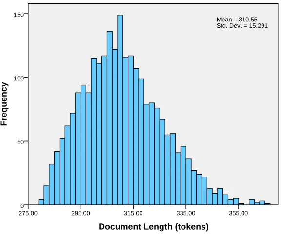
The 10 native languages and the number of texts generated per class are listed in Table 2. In addition to these we also generate 250 control texts written by native

Document Length (tokens)

355.00 335.00

315.00 295.00

275.00

Frequency

150

100

50

0

Mean = 310.55 Std. Dev. = 15.291 …

Figure 3

A histogram of the number of tokens per document in the data set that we generated.

speakers. A histogram of the number of tokens per document is shown in Figure 3. The documents have an average length of 311 tokens with a standard deviation of 15 tokens.

Part-of-Speech Tagset.The ASK corpus uses the Oslo-Bergen tagset,12 _{which has been} developed based on the Norwegian Reference Grammar (Faarlund, Lie, and Vannebo 1997).

Here each POS tag is composed of a set of constituent morphosyntactic tags. For example, the tagsubst-appell-mask-ub-flsignifies that the token has the categories “noun common masculine indefinite plural.” Similarly, the tagsverb-impand verb-presrefer to imperative and present tense verbs, respectively.

Given its many morphosyntactic markers and detailed categories, the ASK data set has a rich tagset with over 300 unique tags.

3.4 The Jinan Chinese Learner Corpus

Growing interest has led to the recent development of the Jinan Chinese Learner Corpus (JCLC; Wang, Malmasi, and Huang 2015), the first large-scale corpus of L2 Chinese consisting of university student essays. Learners from 59 countries are represented and proficiency levels are sampled representatively across beginner, intermediate, and advanced levels. Texts by learners from other Asian countries are disproportionately represented, with this likely being due to geographical proximity and links to China. Again, we constructed raw and generated data sets from this corpus, the former as a standard set-up and the latter to try to mitigate the effects of topic bias, length heterogeneity, and so forth.13

Raw. To construct the raw JCLC data set, for the smaller L1s, we kept all of the documents, and for the larger ones we randomly sampled from among the original documents, in a manner such that the rank order of each language was preserved (e.g., Indonesian was still the most common L1).

Generated.For the generated JCLC data set, we extracted 3.75 million tokens of text from the JCLC in the form of individual sentences. Following the methodology described in the previous section, we combine the sentences from the same L1 to generate texts of 600 tokens on average,14_{creating a set of documents suitable for NLI.}

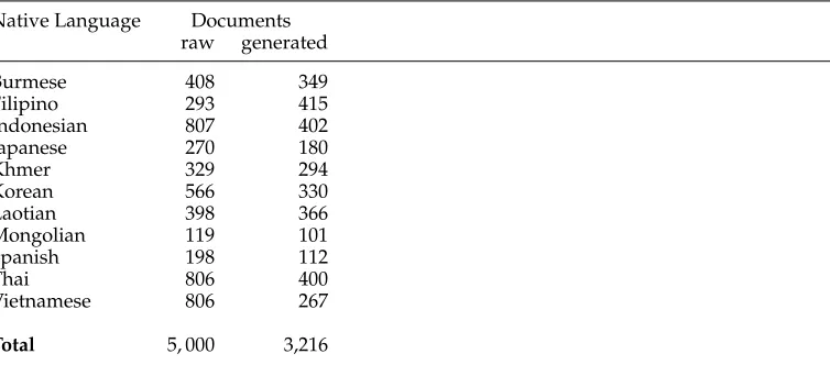
Although there are over 50 L1s available in the corpus, we choose the top 11 lan-guages, shown in Table 3, to use in our experiments. This is based on two considerations. First, although many L1s are represented in the corpus, most have relatively few texts. Choosing the top 11 classes allows us to have a large number of classes and also to ensure that there are sufficient data per-class. Second, this is the same number of classes used in the NLI 2013 shared task, enabling us to draw cross-language comparisons with the shared task results.

12http://tekstlab.uio.no/obt-ny/english/tagset.html.

13 We note that this corpus does not provide topic information at a document level in the metadata, so there is no possibility of balancing raw documents by topic. We also note that in the description by Wang, Malmasi, and Huang (2015) of the JCLC corpus, there is huge variance in the mean text length per class, ranging from 401 to 1,135 tokens. This is reflected across the whole data set, as shown in Figure 1 of Wang, Malmasi, and Huang (2015).

14 A single Chinese character is considered a token.

Table 3

The 11 L1 classes included in the Chinese NLI data set, and the numbers of raw documents and documents we generated for each class.

Native Language Documents raw generated

Burmese 408 349

Filipino 293 415

Indonesian 807 402

Japanese 270 180

Khmer 329 294

Korean 566 330

Laotian 398 366

Mongolian 119 101

Spanish 198 112

Thai 806 400

Vietnamese 806 267

Total 5, 000 3,216

4. Experimental Set-up

In this study we use a supervised multiclass classification approach. The learner texts are organized into classes according to the author’s L1 and these documents are used for training and testing in our experiments. In this section we describe our experimental methodology, including evaluation and the algorithms we use. Our classification fea-tures will be described in Section 5; and the three classification models we create using these algorithms and features are then described in Section 6.

4.1 Evaluation

In the same manner as many previous NLI studies and also the NLI 2013 shared task, we report our results as classification accuracy underk-fold cross-validation, withk=10. In recent years this has become a de facto standard for reporting NLI results. For creating our folds, we used stratified cross-validation, which aims to ensure that the proportion of classes within each partition is equal (Kohavi 1995). For TOEFL11 we also test on the standard test set, which we call TOEFL11-TEST.

We use three baselines to provide lower bounds for accuracy:

r

r

r

consisting of all features used in the data set, as a direct comparator for using an ensemble vs. not using one (as per Tetreault et al. [2012]).

We use additional baselines depending on the corpus, where comparable results by other systems are available.

Oracles, which we describe in Section 6.1.8, will also be used to estimate a potential upper bound for accuracy. We use them to assess how close our models are to achieving

optimal performance. Additionally, we also compare our results against those reported in previous work. These were described earlier in Section 2.

4.2 Statistical Significance Testing

Statistical significance testing in NLP is not universal, and there is not a standard approach to it even among purely classification tasks. To our knowledge the level of significance of differences in various NLI systems has not been previously carried out, so in this section we just note the test we will use to compare the best result from our various approaches against other top results from the literature.

Because we are evaluating the classifier outputs for the same samples, a test for paired nominal data is suitable. We use McNemar’s test (McNemar 1947), a non-parametric method to test for significant differences in proportions for paired nominal data; it has been used widely elsewhere in the machine learning literature (West 2000; Aue and Gamon 2005, for example), and a description of its use in classification tasks is available in Foody (2004).

We note that it does require the entire set of predictions from each system to be compared. Predictions made by all 144 submissions in the 2013 shared task were made available as part of Malmasi, Tetreault, and Dras (2015).15_{For the work described in this} article, Ionescu, Popescu, and Cahill (2014) also kindly provided us with the predictions from their state-of-the-art system, which we also make available.16_{As part of this work,} we also make available the predictions of our best system on the TOEFL11-TESTset.

4.3 Classification Methods

In this work we use a range of classifiers, all of which have been used for text classifi-cation and most of which are standard, although we make some remarks on a couple of them here. All of the learners listed will be used as meta-classifiers, but only SVMs and Logistic Regression will be considered as base learners, as we note subsequently. The learners to be used are:

r

r

r

r

r

r

r

Dirichlet Allocation) (Fisher 1936);

r

2009);

15 Available fromhttp://web.science.mq.edu.au/~smalmasi/resources/nli2013. 16 These two sets of predictions are available at

http://web.science.mq.edu.au/~smalmasi/resources/nli-predictions.

r

r

Multiclass Classification. Some methods such as multinomial logistic regression are in-herently multiclass. Others, such as SVMs, however, are inin-herently binary classifiers. A common way to adapt these binary classifiers for multiclass problems is through a one-vs.-all (OVA) approach, also known as a one-vs.-rest (OVR) approach. Another common alternative is a one-vs.-one (OVO) method that builds N(N₂−1) binary classifiers for all pairwise combinations. For SVMs in the context of NLI, it has been found that the OVR approach works best (Brooke and Hirst 2012b), and our experiments confirmed this. We therefore adopt this approach to multiclassing for all methods that are not already multiclass.

Classifier Output Representation. As we will describe in Section 6, our meta-classifiers are trained on the outputs generated by individual base classifiers, which can be either discrete labels or continuous values.

All classifiers produce discrete label output, which is represented as a one-hot vector of sizeK, the number of classes in the data set. Additionally, some classifiers such as Logistic Regression naturally provide continuous values associated with each of the possibleKclass labels; for some of these the continuous values represent probabilities of the labels, or can be interpreted as some other measure of confidence in the labels. Where available, this output information can also be used to form a vector for classifi-cation. For each input, this would result in aK-element vector where each element is the continuous output associated with a class label. Where it is not available by default, it is sometimes possible to derive a score associated with each label.

SVMs and Logistic Regression. Linear SVM classifiers are a highly robust supervised classification method that has proven to be very effective for text classification (Joachims 1998). Strong theoretical and empirical arguments have been made for the utility of SVMs for text classification, showing that their capabilities are well suited for several properties of text data, including extremely large feature spaces, very high sparsity, and few irrelevant features.

With regard to NLI, post hoc analysis of the 2013 shared task results revealed that many of the top systems, including the winning entry, followed two broad patterns: they used SVM classifiers along with frequency-based feature values. We thus consider this as one possibility for our base classifiers.

We note that SVM is a margin-based classifier and does not output probability estimates for each class label as a part of the classification. However, there are methods to map the outputs to probabilities based on the signed distance to the separating hyperplane (Platt 2000); we use this technique in this article.

We also use RBF-kernel SVMs, but only for the meta-classifier. Hsu et al. (2003, Appendix C) have examined the way in which this type of kernel may work poorly for large feature spaces, which makes it unsuitable for the base classifier, but the meta-classifier will use many fewer features.

Logistic regression is a type of linear regression model where the dependent vari-ables are categorical. Although high-dimensional input poses a challenge for these models (Genkin, Lewis, and Madigan 2007), this issue can be addressed to some degree using regularization methods (Zhu and Hastie 2004).

Logistic regression was also popular in the shared task, so we consider that as an alternative to linear SVMs for our base classifier, with both L1 and L2 regularization.

This algorithm is inherently multiclass, meaning that OVA and OVO approaches are not required. The logistic regression classifier is also probabilistic and provides continuous probability estimates for each class label.

LDA/QDA.Unlike the other classifiers, LDA and QDA are not widely used in NLP. However, we investigate them in this work because they have been successfully used for classification elsewhere—Liu and Wechsler (2002), for example, in vision—but more particularly because the body of work that came out of the field of SLA (Jarvis and Crossley 2012) used it extensively.

LDA is a classic learning algorithm, dating to Fisher (1936); an accessible explana-tion is given in Hastie, Tibshirani, and Friedman (2009). Like naive Bayes, LDA and QDA are based on models for the class-conditional densities; whereas naive Bayes uses non-parametric class density estimates that are the products of marginal densities (i.e., assuming inputs are conditionally independent with respect to class), LDA and QDA use multivariate Gaussian densities. Where classes are assumed to have a common covariance matrix, this gives the special case of LDA, where the decision boundary becomes a hyperplane. QDA is the case where the assumption of common covariance across classes is not made, resulting in a quadratic decision surface. Unlike LDA, how-ever, it makes no assumption about equal class covariances, allowing them to be class-specific. Both LDA and QDA are inherently multiclass. Hastie, Tibshirani, and Friedman (2009, page 111) note that they have performed well on a range of classification tasks and comment that “whatever exotic tools are the rage of the day, we should always have available these two simple tools.”

5. Features

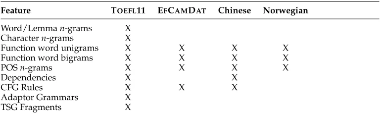
As its focus is on classifier architecture, this study just utilizes a standard set of NLI features used in previous work, as noted in, for example, the overview of the systems in the NLI shared task of 2013 (Tetreault, Blanchard, and Cahill 2013). We combine these various feature types because it has been shown that both lexical and syntactic features each capture diverse types of information that are complementary (Malmasi and Cahill 2015). Different feature types are extracted for each of our data sets, as shown in Table 4.

Table 4

An overview of the features used for each data set.

Feature TOEFL11 EFCAMDAT Chinese Norwegian

Word/Lemman-grams X

Charactern-grams X

Function word unigrams X X X X

Function word bigrams X X X X

POSn-grams X X X X

Dependencies X X

CFG Rules X X X

Adaptor Grammars X

TSG Fragments X

The feature types for each data set were chosen based on properties of the data set and the availability of NLP resources for the L2.

For stylistic classification tasks like NLI, these content-based features can only be used if the training data are balanced for topic. Otherwise, topic balance may impact the results and artificially inflate accuracy (Malmasi and Dras 2017a). Accordingly, we only use these features for our experiments with TOEFL11, which is balanced for topic. The NLP tools used to extract adaptor grammar and Tree Substitution Grammar (TSG) fragment features are only available for English. The paucity of NLP tools for Norwegian and the lack of topic balance in the data also limited our features to those manually annotated in the data set.

We remark here that the key goal of this article is to systematically evaluate ensem-ble architectures, not features: We will be comparing the performance of our models withina particular experimental set-up (a single data set for within-corpus, two data sets for cross-corpus) and notacrossthese.

The remainder of this section describes the feature types listed in Table 4.

Word, Lemma, and Character n-grams. For TOEFL11, we extract content word unigrams and bigrams, lemma unigrams and bigrams, and character uni/bi/trigrams. For stylis-tic classification tasks like NLI, these content-based features can artificially boost perfor-mance through detecting topic-related, rather than NLI-related, clues (Koppel, Schler, and Argamon 2009): As noted in Section 2.2 and Section 3.1, TOEFL11 was constructed as the first corpus used for NLI that was topic-balanced to minimize this issue. Accord-ingly, we only use these features for our experiments with TOEFL11.

As discussed in more detail in Malmasi and Dras (2015), we do not use these features for EFCAMDAT, aiming to minimize topic-related clues: They noted that, for a classifier using word unigrams, the topic 15 features contained strong content-based clues (e.g., the words Germany, Berlin, Hamburg, Frankfurt, and Munich for German; and Saudi,Arabia,Arabic,Mohammed, and Alifor Arabic). Although it is not possible to eliminate the topic bias,17_{omitting these features reduces it. And as Brooke and Hirst} (2011) note, the use of cross-corpus evaluation is another technique for minimizing the effect of topical clues.

Function Words. In contrast to content words, function words (e.g., articles, deter-miners, conjunctions and auxiliary verbs) do not have any thematic meaning them-selves, but rather can be seen as indicating the grammatical relations between other words; consequently, they have been widely used in stylistic classification tasks. In this work, the English word list was obtained from the Onix Text Retrieval Toolkit.18 _For Norwegian we used a list of 176 function words obtained from the distribution of the Apache Lucene search engine software.19 _{This list includes stop words for the Bokm˚al} variant of the language and contains entries such as hvis [whose], ikke [not], jeg [I], s˚a [so], and hj˚a [at]. We also make this list available on our Web site.20 For Chinese, we utilize the function word list described in Malmasi and Dras (2014b).

17 It is true that other features can still detect topic bias: Brooke and Hirst (2011) showed that the ICLE corpus suffered from this, as, for example, the fact that French texts were more about philosophy and religion, whereas Japanese texts were more about personal experiences, such as language learning and travel, had related register differences that could be detected by non-content features.

18http://www.lextek.com/manuals/onix/stopwords1.html. 19https://github.com/apache/lucene-solr.

20http://web.science.mq.edu.au/~smalmasi/data/norwegian-funcwords.txt.

In addition to single function words, we also extract function word bigrams, as described by Malmasi, Wong, and Dras (2013). Function word bigrams are a type of wordn-gram where content words are skipped: They are thus a specific subtype of the skipgrams discussed by Guthrie et al. (2006). For example, the sentence “We should all start taking the bus” would be reduced to “we should all the,” from which we would extract then-grams.

Part-of-Speechn-grams. The TOEFL11 data was tagged using two different tagsets: the Penn Treebank tagset (PTB) and the CLAWS tagset, which has been shown to perform well for NLI (Malmasi, Wong, and Dras 2013). The tagging was performed using the Stanford CoreNLP software21 (Manning et al. 2014) and the Robust Accurate Statistical Parsing (RASP)22 system (Briscoe, Carroll, and Watson 2006), respectively. Detailed information and comparison between the tagsets, including a discussion of their effects on NLI accuracy, can be found in Malmasi and Dras (2017a, Section 9). The EFC data were tagged using only the PTB tagset in order to replicate the baseline system against which we evaluate our results.

We also used Stanford CoreNLP for Chinese. We did not use any NLP tools for Norwegian as the corpus we use is already annotated with POS tags.

We extracted POS n-grams of order 1–3, which have been shown to be useful for NLI (Malmasi, Wong, and Dras 2013). Previous work and our experiments showed that sequences of size 4 or greater achieve lower accuracy, possibly because of data sparsity, so we do not include them.

Adaptor Grammar Collocations. Following Wong, Dras, and Johnson (2012), for the TOEFL11 data we include arbitrary lengthn-gram collocations discovered by an adaptor grammar. We use the specific features obtained by Wong, Dras, and Johnson (2012), both the pure POSn-grams as well as the better-performing mixtures of POS and function words.

Stanford Dependencies. For English and Chinese, we use Stanford dependencies as a syntactic feature: For each text we extract all the basic dependencies returned by the Stanford parser (de Marneffe, Maccartney, and Manning 2006). We then generate all the variations for each of the dependencies (grammatical relations) by substituting each lemma with its corresponding POS tag. For instance, a grammatical relation of det(knowledge, the)yields the following variations:det(NN, the),det(knowledge, DT), anddet(NN, DT).

CFG Rules. For English and Chinese, we obtain a constituent-based parse using the Stanford parser, and extract the production rules that constitute those trees to use as features.

Tree Substitution Grammar Fragments.TSG fragments were proposed by Swanson and Charniak (2012) as another type of syntactic feature for NLI that captures a broader syntactic context than the single-level fragments of phrase-structure trees that constitute the CFG rules. We only extract TSG fragments for the TOEFL11 data as they include lexical terminal nodes.

21http://nlp.stanford.edu/software/corenlp.shtml. 22http://users.sussex.ac.uk/~johnca/rasp/.

6. Classification Models

We conduct a set of three experiments, each based on different ensemble structures that we describe in this section. The first model is based on a traditional parallel ensemble structure and the second model examines meta-classification using classifier stacking. The third and final model is a hybrid approach, building an ensemble of meta-classifiers.

6.1 Ensemble Classifiers

The most common ensemble structure, as described earlier in Section 2.1, relies on a set of base classifiers whose decisions are combined using some predefined method. This is the approach for our first model.

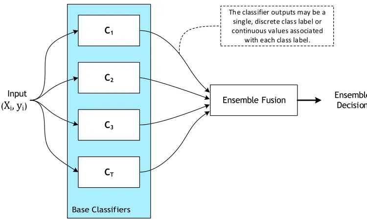
Such systems often use a parallel architecture, as illustrated in Figure 4, where the classifiers are run independently and their outputs are aggregated using a fusion method. The first part of creating an ensemble is generating the individual classifiers. Various methods for creating these ensemble elements have been proposed. These involve using different algorithms, parameters, or feature types; applying different pre-processing or feature scaling methods; and varying (e.g., distorting or resampling) the training data. (See Dietterich [2000] for a more detailed discussion of several methods.) For example, Bagging (bootstrap aggregating) is a commonly used method for ensemble generation (Breiman 1996) that can create multiple base classifiers. It works by creating multiple bootstrap training sets from the original training data and a separate classifier is trained from each set. The generated classifiers are said to be diverse because

C1

C2

C3

CT

Ensemble Fusion Ensemble _Decision

Input (

X

, y

The classifier outputs may be a single, discrete class label or continuous values associated

with each class label.

Figure 4

An example of a parallel ensemble classifier architecture whereTindependent classifiers provide predictions, which are then fused using a rule-based ensemble combination method. The class labels for the input,yi, are only available during training or cross-validation. In this

work the input vectorXifor each classifier is a distinct vector based on a single feature type.

each training set is created by sampling with replacement and contains a random subset of the original data.Boosting(e.g., with the AdaBoost algorithm) is another method where the base models are created with different weight distributions over the training data with the aim of assigning higher weights to training instances that are misclassified (Freund and Schapire 1996).

In our first model we follow the same approach as previous NLI research and train each classifier on a different feature type.23However, our other models make use of the boosting and bagging techniques, which will be discussed in later sections. As noted in Section 4.3, we consider linear SVMs and logistic regression for these base classifiers.

The second part of ensemble design is choosing a combination or fusion rule to aggregate the outputs from the various learners; this is discussed in the next section. Most NLI research to date has not compared different types of such combiners and we aim to evaluate a number of different strategies.

6.1.1 Ensemble Fusion Methods.Once it has been decided how the set of base classifiers will be generated, selecting the classifier combination method is the next fundamental design question in ensemble construction.

The answer to this question depends on what output is available from the indi-vidual classifiers. The two different output types were discussed earlier in Section 4.3. Some combination methods are designed to work with class labels, assuming that each learner outputs a single class label prediction for each data point. Other methods are designed to work with class-based continuous output, requiring that for each instance every classifier provide a measure of confidence24 _{for each class label. These outputs} may correspond to probabilities for each class and consequently sum to 1 over all the classes. If an algorithm can provide both types of output, then all the methods can be tested. This is the case for the SVM and logistic regression classifiers we will work with. These methods are usually based on some predefined rule or logic and cannot be trained. This can be considered an advantage, allowing them to be implemented and used without additional training of domain-specific combination models. On the other hand, they may not be able to exploit domain-specific trends and patterns in the input data.

Although a number of different fusion methods have been proposed and tested, there is no single dominant method (Polikar 2006). The performance of these methods is influenced by the nature of the problem and available training data, the size of the ensemble, the base classifiers used, and the diversity between their outputs. This is an important motivation for comparatively assessing these methods on NLI data.

The selection of this method is often done empirically. Many researchers have com-pared and contrasted the performance of combiners on different problems, and most of these studies—both empirical and theoretical—do not reach a definitive conclusion (Kuncheva 2014, page 178).

In the same spirit, we experiment with several classifier fusion methods that have been widely applied and discussed in the machine learning literature. Our selected methods are described in the following paragraphs; a variety of other methods exist and the interested reader can refer to the thorough exposition by Polikar (2006).

23 An alternative is to train each classifier on a subspace of the entire feature set that includes all types. 24 For example, an estimate of the posterior probability for the class label.

Decision profile COMBINER

Class label MAX

D₁ D₂

… Feature

vector

Classifiers

DL

AVERAGE

FIGURE 5.5 Operation of the average combiner.

Represented by the average combiner, the category of simple nontrainable combiners is described in Figure 5.4, and illustrated diagrammatically in Figure 5.5. These combiners are called nontrainable, because once the individual classifiers are trained, their outputs can be fused to produce an ensemble decision, without any further training.

◻◼

The following example helps to clarify simple combiners. Let c=3 and L=5. Assume that for a certainx

DP(x)=

⎡ ⎢ ⎢ ⎢ ⎢ ⎣

0.1 0.5 0.4 0.0 0.0 1.0 0.4 0.3 0.4 0.2 0.7 0.1 0.1 0.8 0.2

⎤ ⎥ ⎥ ⎥ ⎥ ⎦

. (5.20)

Applying the simple combiners column wise, we obtain:

Combiner _𝜇1(x) 𝜇2(x) 𝜇3(x)

Average 0.16 0.46 0.42

Minimum 0.00 0.00 0.10

Maximum 0.40 0.80 1.00

Median 0.10 0.50 0.40

40% trimmed mean 0.13 0.50 0.33

Product 0.00 0.00 0.0032

Figure 5

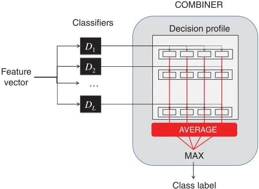
An example of a mean probability combiner. The feature vector for a sample is input toL different classifiers, each of which output a vector of confidence probabilities for each possible class label. These vectors are combined to form the decision profile for the instance that is used to calculate the average support given to each label. The label with the maximum support is then chosen as the prediction. Image reproduced from Kuncheva (2014, Fig. 5.5) with permission.

6.1.2 Plurality Voting.Each classifier votes for a single class label. The votes are tallied and the label with the highest number of votes wins.25 _{Ties are broken arbitrarily. This} method is simple and does not have any parameters to tune. An extensive analysis of the method and its theoretical underpinnings can be found in Kuncheva (2004, page 112).

6.1.3 Mean Probability Rule. The probability estimates for each class, provided by each individual classifier, are summed and the class label with the highest average probabil-ity is the winner. This is illustrated in Figure 5. This is equivalent to the probabilprobabil-ity sum combiner, which does not require calculating the average for each class. An important aspect of using probability outputs in this way is that a classifier’s support for the true class label is taken into account, even when it is not the predicted label (e.g., it could have the second highest probability). This method has been shown to work well on a wide range of problems and, in general, it is considered to be simple, intuitive, stable (Kuncheva 2014, page 155), and resilient to estimation errors (Kittler et al. 1998), making it one of the more robust combiners discussed in the literature.

6.1.4 Median Probability Rule.Given that the mean probability used in the mean proba-bility rule is sensitive to outliers, an alternative is to use the median as a more robust estimate of the central value (Kittler et al. 1998). Under this rule, each class label’s estimates are sorted and the median value is selected as the final score for that label. The label with the highest median value is picked as the winner. As with the mean

25 This differs with amajorityvoting combiner, where a label must obtain over 50% of the votes to win. However, the names are sometimes used interchangeably.

combiner, this method measures the central tendency of support for each label as a means of reaching a consensus decision.

6.1.5 Product Rule.For each class label, all of the probability estimates are multiplied together to create the label’s final estimate (Polikar 2006, page 37). The label with the highest estimate is selected. This rule can theoretically provide the best overall estimate of posterior probability for a label, assuming that the individual estimates are accurate. A trade-off here is that this method is very sensitive to low probabilities: A single low score for a label from any classifier will essentially eliminate that class label.

6.1.6 Highest Confidence. In this simple method, the class label that receives the vote with the largest degree of confidence is selected as the final prediction (Kuncheva 2014, page 150). In contrast to the previous methods, this combiner disregards the consensus opinion and instead picks the prediction of the expert with the highest degree of confidence.

6.1.7 Borda Count.This method works by using each classifier’s confidence estimates to create a ranked list of the class labels in order of preference, with the predicted label at rank 1. The winning label is then selected using the Borda count26 _{algorithm (Ho,} Hull, and Srihari 1994). The algorithm works by assigning points to labels based on their ranks. If there areNdifferent labels, then each classifier’s preferences are assigned points as follows: the top-ranked label receivesNpoints, the second place label receives N−1 points, third place receives N−2 points, and so on, with the last preference receiving a single point. These points are then tallied to select the winner with the highest score.

The most obvious advantage of this method is that it takes into account all of each classifier’s preferences, making it possible for a label to win even if another label received the majority of the first preference votes.

6.1.8 Oracle Combiners.Our final set of combiners are designed to assist with assessing the potential performance upper bound that could be achieved by a system, given a set of classifiers. As such, they are primarily used for evaluation in the same manner that baselines help determine the lower bounds for performance. These combiners cannot be used to make predictions on unlabeled data.

One possible approach to estimating an upper-bound for classification accuracy, and one that we use here, is the use of an “oracle” combiner. This method has previously been used to analyze the limits of majority vote classifier combination (Kuncheva, Bezdek, and Duin 2001). An oracle is a type of multiple classifier fusion method that can be used to combine the results of an ensemble of classifiers that are all used to classify a data set.

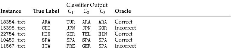
The oracle will assign the correct class label for an instance if at least one of the constituent classifiers in the system produces the correct label for that data point. Some example oracle results for an ensemble of three classifiers are shown in Table 5. The probability of correct classification of a data point by the oracle is:

POracle=1−P(All Classifiers Incorrect)

26 This method is generally attributed to Jean-Charles de Borda (1733–1799), but evidence suggests that it was also proposed by Ramon Llull (1232–1315).

Table 5

Example oracle results for an ensemble of three classifiers.

Classifier Output

Instance True Label C1 C2 C3 Oracle

18354.txt ARA TUR ARA ARA Correct

15398.txt CHI JPN JPN KOR Incorrect

22754.txt HIN GER TEL HIN Correct

10459.txt SPA SPA SPA SPA Correct

11567.txt ITA FRE GER SPA Incorrect

Oracles are usually used in comparative experiments and to gauge the performance and diversity of the classifiers chosen for an ensemble (Kuncheva 2002; Kuncheva et al. 2003). They can help us quantify thepotentialupper limit of an ensemble’s performance on the given data and how this performance varies with different ensemble configura-tions and combinaconfigura-tions.

To account for the possibility that a classifier may predict the correct label essentially by chance (with a probability determined by the random baseline) and thus exaggerate the oracle score, we also use an Accuracy@Ncombiner. This method is inspired by the “Precision atk” metric from Information Retrieval (Manning, Raghavan, and Sch ¨utze 2008), which measures precision at fixed low levels of results (e.g., the top 10 results). Here, it is an extension of the Plurality vote combiner, where instead of selecting the label with the highest votes, the labels are ranked by their vote counts and an instance is correctly classified if the true label is in the topNranked candidates.27 Another way to view it is as a more restricted version of the Oracle combiner that is limited to the topNranked candidates in order to minimize the influence of a single classifier having chosen the correct label by chance. In this study we experiment withN=2 and 3. We also note that settingN=1 is equivalent to the Plurality voting method and settingN to the number of class labels is equivalent to the Oracle combiner.

6.2 Meta-Classifiers

While the combination methods in our first model are not trainable, other more sophis-ticated ensemble methods that rely on meta-learning use a stacked architecture where the output from a first layer of classifiers is fed into a second-level meta-classifier, and so on. For our second model we expand our methodology to such a meta-classifier, also referred to asclassifier stacking(Wolpert 1992).

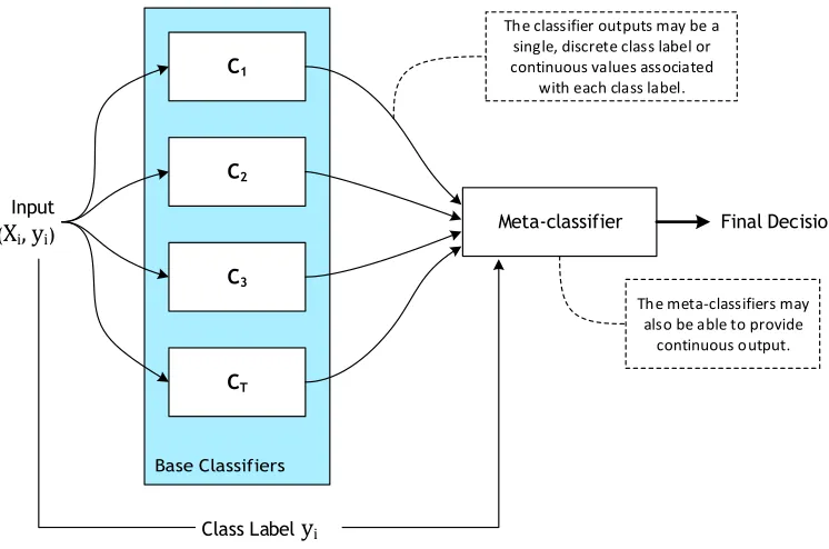
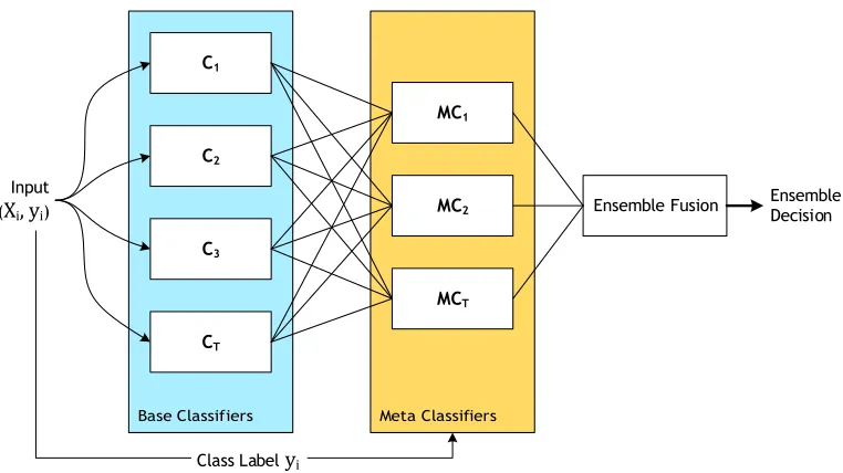
A meta-classifier architecture is composed of an ensemble of base classifiers, just as in our first model. A key difference is that instead of using a rule-based fusion method, the individual classifier outputs, along with the training labels, are used to train a second-level meta-classifier. This second meta-learner serves to predict the final decision for an input, given the decisions of the base classifiers. This set-up is illustrated in Figure 6.

27 In case of ties, we choose randomly from the labels with the same number of votes.

C1

C2

C3

CT

Meta-classifier Final Decision

Input (

X

, y

Class Label

y

The classifier outputs may be a single, discrete class label or continuous values associated

with each class label.

The meta-classifiers may also be able to provide

continuous output.

Figure 6

An example architecture for a meta-classifier. The outputs generated by the set ofTbase classifiers, along with the labels of the training data, are used to train a meta-learner that can predict the final decision for an input. This meta-classifier attempts to learn from the collective knowledge represented by the ensemble of base classifiers and may be able to learn and exploit regularities in their output. The class labels for the input are only available during training or cross-validation. In this work the input vectorXifor each base classifier is a distin