Munich Personal RePEc Archive
Estimation and Inference in
Functional-Coefficient Spatial
Autoregressive Panel Data Models with
Fixed Effects
Sun, Yiguo and Malikov, Emir
University of Guelph, Auburn University
2017
Online at
https://mpra.ub.uni-muenchen.de/83671/
Estimation and Inference in Functional-Coefficient Spatial
Autoregressive Panel Data Models with Fixed Effects
∗Yiguo Sun
Department of Economics and Finance, University of Guelph, Guelph, ON N1G2W1, Canada
Emir Malikov
Department of Agricultural Economics, Auburn University, Auburn, AL 36849, USA
First Draft: December 25, 2015 This Draft: July 15, 2017
Abstract
This paper develops an innovative way of estimating a functional-coefficient spatial autoregres-sive panel data model with unobserved individual effects which can accommodate (multiple) time-invariant regressors in the model with a large number of cross-sectional units and a fixed number of time periods. The methodology we propose removes unobserved fixed effects from the model by transforming the latter into a semiparametric additive model, the estimation of which however does not require the use of backfitting or marginal integration techniques. We derive the consistency and asymptotic normality results for the proposed kernel and sieve estimators. We also construct a consistent nonparametric test to test for spatial endogeneity in the data. A small Monte Carlo study shows that our proposed estimators and the test statistic exhibit good finite-sample performance.
Keywords: First Difference, Fixed Effects, Hypothesis Testing, Local Linear Regression, Non-parametric GMM, Sieve Estimator, Spatial Autoregressive, Varying Coefficient
JEL Classification: C12, C13, C14, C23
1
Introduction
Sun, Carroll & Li (2009) and Lin, Li & Sun (2014) study the following semiparametric functional-coefficient fixed-effects panel data model:
yit =gi′θ(zit) +x′itβ(zit) +µi+uit, i= 1, . . . , n, t= 1, . . . , T, (1.1) where yit is the (scalar) outcome variable of interest; gi and xit are the invariant and time-varying explanatory variables of dimensionsdganddx, respectively;zitis a continuously distributed univariate random variable; andθ(·) andβ(·) are thedg×1 anddx×1 vectors of unknown functions to be estimated. The unobserved fixed effectsµiare allowed to correlate with the strictly exogenous covariatesgi,xit andzit, but are assumed to be uncorrelated with the idiosyncratic erroruit, which isi.i.d. with zero mean and finite varianceσ2
u. Both Sun et al. (2009) and Lin et al. (2014) restrict their models to the case of dg ≤1.
The above semiparametric model has proven to be a popular specification among practitioners. Not only can the model in (1.1) be conveniently applied to reduce the “curse-of-dimensionality” problem, but it also nests purely nonparametric fixed-effects panel data models as well as partially linear fixed-effects panel data models studied by Henderson, Carroll & Li (2008), Qian & Wang (2012) and Li & Liang (2015), who all however focus on a rather restrictive case of dg = 0.
In this paper, we seek to generalize model (1.1) further to the case with spatial dependence in the data. We do so by including the spatial lag of the outcome variable as an additional explanatory variable and allowing the corresponding spatial multiplier to vary with respect to the contextual covariatezit. That is, we consider the following functional-coefficient spatial autoregressive (SAR) fixed-effects panel data model:
yit=ρ(zit)
X
j6=i
wijyjt+g′iθ(zit) +x′itβ(zit) +µi+uit, i= 1, . . . , n, t= 1, . . . , T, (1.2)
where Pj6=iwijyjt is called the “spatial lag” term; wij is the (i, j)-th element of an n×n pre-determined non-stochastic time-invariant spatial weighting matrix W0 such that wii = 0 for all
i= 1, . . . , n; andyitis spatially stationary.1 Further,ρ(·) is usually referred to as the “spatial mul-tiplier” or “spatial lag parameter”, which is an unknown function to be estimated. For instance, when the SAR model is game-theoretically rationalized as a “reaction function” (e.g., Brueckner, 2003), the spatial multiplierρ(·) can be conveniently interpreted as the “reaction” parameter, which our model permits to meaningfully vary with some contextual factorzit. Since the spatial multiplier captures the direct impact of other units’ actions/outcomes on the ith unit’s action/outcome, ex-tending (1.1) to model (1.2) enables us to test whether there is spatial/economic externality across individual units. Also note that, when ρ(z)≡ρ0, θ(z)≡0dg and β(z)≡β0, our semiparametric
model (1.2) collapses to Lee & Yu’s (2010a) fully parametric SAR fixed-effects panel data model. Some potential applications of our model, for instance, include the estimation of growth mod-els that explicitly account for technological interdependence between countries in the presence of spillover effects. Such a technological interdependence is usually formulated in the form of spa-tial externalities (e.g., see Ertur & Koch, 2007). However, the intensity of knowledge spillovers is naturally expected to greatly depend on institutional and cultural compatibility of neighboring countries (Kelejian, Murrell & Shepotylo, 2013). Our functional-coefficient model presents a prac-tical method to allow for such indirect effects of institutions on the degree of spatial dependence in the cross-country conditional convergence regressions via a contextual variablezit. The estimation
of hedonic house price functions is another application, where it is imperative to allow for potential spatial dependence in the data. House prices are widely believed to be spatially autoregressive because residential property values tend to reflect shared local amenities as well as observed and unobserved neighborhood characteristics. While these characteristics can be partly controlled for using locality fixed effects, such an approach may be unsatisfactory since it does not let charac-teristics of neighboring houses affect the price of a given house (Anselin & Lozano-Gracia, 2009). However, by including the spatial lag in a house pricing function, one is able to accommodate such cross-neighbor effects.
In recent decades, the econometric literature has seen a rapid development in the theory of non-parametric estimation and testing of fixed-effects panel data models. For instance, see Sun, Zhang & Li (2015) for an excellent survey on the nonparametric panel data analysis. However, the intro-duction of nonparametric structure to models with spatial dependence (and spatial autoregressive models, in particular) in the panel data setup still lacks enough attention and progress, although significantly more visible advances have been made in the development of parametric spatial models (e.g., Lee & Yu, 2010a,b, 2012, 2014; Yu, de Jong & Lee, 2012). Our work therefore aims to fill this research gap in the literature.
Few existing nonparametric studies, all of which focus on a purely cross-sectional setup, include the works of Su & Jin (2010), Su (2012) and Zhang (2013), who consider a Robinson-type partially linear semiparametric SAR model, whereas Sun, Yan, Zhang & Lu (2014) and Malikov & Sun (2017) study fully and/or partially linear functional-coefficient SAR models. The spatial autoregressive models in which spatial weights are specified in the form of unknown nonparametric functions of some geographic or economic distance are examined by Pinkse, Slade & Brett (2002) and Sun (2016).
For a large n and fixed T, we develop an innovative way of estimating model (1.2). We first propose a two-stage kernel estimation method to estimate ρ(·) and β(·), after removing the un-observed fixed effects from the model via first differencing. Our approach transforms the model into a semiparametric additive panel data model from which a consistent estimator is usually con-structed using either the backfitting (Henderson et al., 2008; Mammen, Støve & Tjøstheim, 2009; Li & Liang, 2015) or marginal integration techniques (Qian & Wang, 2012).2 Unlike a more con-ventional model (1.1), our model of interest in (1.2) naturally suffers from the endogeneity problem due to the presence of the spatial lag term in the equation. We therefore resort to a nonparametric instrumental variable approach in order to construct consistent estimators of the unknown coeffi-cient curvesρ(·) and β(·). However, when based on both localized linear and quadratic moments, the nonparametric GMM estimator has no analytic expression. Consequently, both the backfitting and marginal integration techniques can be computationally challenging in the calculation of such an estimator for model (1.2). Therefore, we propose a new estimator that is significantly simpler to implement than the backfitting and marginal integration estimators.
Having consistently estimated ρ(·) and β(·) at the conventional nonparametric convergence rate in the second stage, we next propose a third-stage sieve estimator to consistently estimate unknown functional curves θ(·) for time-invariant regressors gi. Importantly, the estimator we propose in this paper can be used to estimate functional coefficients θ(·) even when the number of time-invariant regressors is greater than one, i.e., dg > 1. The methodology that we develop can also be used to estimate the traditional functional-coefficient fixed-effects panel data models with time-invariant covariates like the one in (1.1). This makes a significant improvement over the existing estimation methods that are applicable to the case ofdg ≤1 only (as in Sun et al., 2009).
2Where all these articles consider purely nonparametric fixed-effects panel data models with exogenous covariates
Given that our semiparametric spatial autoregressive model (1.2) nests a more traditional functional-coefficient fixed-effects model in (1.1) as a special case, one may naturally wish to for-mally discriminate between the two models. Therefore, we also propose a consistent residual-based
L2-type test statistic to test for relevance of the spatial lag term in the model. The proposed is, essentially, the test for spatial endogeneity. Our specification test belongs to the family of similar nonparametric residual-based tests considered for independent data (e.g., Zheng, 1996; Li & Wang, 1998), weakly dependent time series data (e.g., Fan & Li, 1999; Li, 1999), integrated time series data (e.g., Wang & Phillips, 2012; Sun, Cai & Li, 2015) and, more recently, for spatial data (e.g., Su & Qu, 2017; Malikov & Sun, 2017).
The rest of the paper is organized as follows. Section 2 explains the model of interest along with the spatial stationarity condition. We derive the consistency and asymptotic normality results for the first-difference kernel estimator of ρ(·) and β(·) in Section 3, whereas the limiting results for a sieve estimator of θ(·) are discussed in Section 4. Section 5 contains a further discussion of the estimation issues. Section 6 presents a consistent nonparametric test statistic to test for the presence of spatial endogeneity in the model. Section 7 reports a small Monte Carlo simulation study to asses the small sample performance of our proposed estimators and the test statistic. We conclude in Section 8. All mathematical proofs are relegated to the Appendix.
Before anything else, we summarize our notation. Boldface letters are reserved for vectors and matrices. (i) Throughout this paper, we denote an [n(T−1)]×dω matrixω =[ω′2, . . . ,ω′T]
′
with an n×dω vectorωt= [ω1t, . . . ,ωnt]′ for any t= 2, . . . , T, whereωit is adω×1 vector. (ii) Let iT be a T×1 vector of ones,0q be a q×1 vector of zeros, Im be anm×m identity matrix and0q×p be a q ×p zero matrix. (iii) k·k refers to the Euclidian norm, and kAk1 = max1≤j≤nPni=1|aij| and kAk∞ = max1≤i≤nPnj=1|aij| are the column and row sum matrix norms, respectively. (iv) Letλj(A),λmin(A) and λmax(A) respectively be thejth, smallest and largest eigenvalue of some
m×m matrixA= (aij)i,jm=1, and kAksp= maxkωk=1,ω6=0kAωk=λ1max/2 (A′A) defines the spectral norm. For any vector a, we see kak=kaksp. (v) We denote As =A+A′ for any square matrix
A. (vi)An=Oe(1) means that each and every element of a random matrixAn is of order Op(1) notop(1). (vii) An=d Bn means that An and Bn have the same distribution asymptotically. (viii) We useC to denote a generic constant that can take different values at different places.
2
The Model
We rewrite model (1.2) in matrix form:
yt=ρ(zt)W0yt+g′θ(zt) +φ′tβ(zt) +µ+ut, t= 1, . . . , T, (2.1) where ρ(zt) = diag{ρ(z1t), . . . , ρ(znt)} is an n×n diagonal matrix of spatial autoregressive pa-rameter functions;β(zt) =β(z1t)′, . . . ,β(znt)′′andθ(zt) =θ(z1t)′, . . . ,θ(znt)′′ are (ndx)×1 and (ndg)×1 vectors of functional coefficients, respectively; φt= diag{x1t, . . . ,xnt} is a (ndx)×n matrix; g = diag{g1, . . . ,gn} is a (ndg)×n matrix; and µ= [µ1, . . . , µn]′ is an n×1 vector of unobserved individual-specific fixed effects. The reduced form of model (2.1) is given by
yt=Sn(zt)g′θ(zt) +φ′tβ(zt) +µ+ut, t= 1, . . . , T (2.2) provided that Sn(zt) = [In−ρ(zt)W0]−1 exists.3 This means that, if
max
1≤j≤n,1≤t≤T|λj{In−ρ(zt)W0}|<1 (2.3)
3By Property 19.15 in Seber (2008, p.421), P∞ i=0A
i
holds almost surely, model (2.2) can be rewritten as
yt=
∞
X
k=0
[ρ(zt)W0]kg′θ(zt) +φ′tβ(zt) +µ+ut, t= 1, . . . , T. (2.4)
For any given t, condition (2.3) implies that the spatial weight [ρ(zt)W0]k becomes smaller in magnitude and less important askincreases. This is analogous to the time-series case of an AR(1) process, e.g.,st=ρst−1+vt, becomes stationary if|ρ|<1, under which conditionst=P∞k=0ρkvt−k. Hence, we say that{yit}isspatially stationaryif (2.3) holds true. Throughout this paper, we assume (2.3) holds. Further discussion of this condition is delayed until Section 5.2.
Next, we note that, in the presence of unobserved fixed effects µ, the functional coefficients
θ(zit) of time-invariant regressors gi are not identifiable fromθ0+θ1(zit), whereθ0 is a vector of constants. Therefore, we normalize these coefficients such that θ(0) = 0dg holds true. This is a
reasonable normalization, sinceg′
iθ0 can always be attributed to time-invariant fixed effects.
3
The First-Difference Kernel Estimator of
ρ
(
z
)
and
β
(
z
)
We propose a two-stage kernel estimation method to estimate model (1.2), removing unobserved fixed effects from the model via the first-difference transformation. We opt to cancel fixed effects out by transforming the model as opposed to “concentrate” them out by employing Sun et al.’s (2009) smoothed dummy variable approach due to infeasibility of the latter in the GMM setup.4
Define two (dx+ 1)×1 vectors: mit =hPj6=iwijyjt,x′it
i′
and γ(zit) = [ρ(zit),β(zit)′]′. Then, applying the first-difference transformation to model (1.2) gives
∆yit=g′i[θ(zit)−θ(zi,t−1)]+m′itγ(zit)−m′i,t−1γ(zi,t−1)+∆uit, i= 1, . . . , n, t= 2, . . . , T (3.1) where ∆yit=yit−yi,t−1 and ∆uit=uit−ui,t−1.
Further, since the spatial lag term in (1.2) is endogenous, we assume there exist dq ≥ 1 valid instruments for Pj6=iwijyjt denoted byqit such that
E[qituis|xi,zi,gi] =0dq ∀i, s, t almost surely, (3.2)
wherexi = [x′i1, . . . ,x′iT]′ and zi = [zi1, . . . , ziT]′, which implies that qit is strictly exogenous. Applying the Taylor expansion toθ(zit) andγ(zit) at an interior pointz1 and toθ(zi,t−1) and γ(zi,t−1) at an interior pointz26=z1, we approximate (3.1) by
∆yit ≈ g′i[θ(z1)−θ(z2)] +m′itγ(z1)−mi,t′ −1γ(z2) + ∆uit
= g′iθ˙(z) +ξ′m′itγ(z) + ∆uit (3.3)
for a given (i, t) such that|zit−z1|=o(1) and |zi,t−1−z2|=o(1), wherez= [z1, z2]′,ξ = [1,−1]′, mit = diag{mit,mi,t−1}, ˙θ(z) = θ(z1)−θ(z2) and γ(z) =γ(z1)′,γ(z2)′′. Note that, due to the time invariance ofgi, we can only identify ˙θ(z) and notθ(z1) andθ(z2) individually.
Equations (3.2) and (3.3) imply the following localized orthogonal moment conditions:
EhQit
∆yit−gi′θ˙(z)−ξ′m′itγ(z)
kit(h,z)
i
≈0d (3.4)
fori= 1, . . . , n,t= 2, . . . , T, whered=dg+2 (dq+dx),Qit=gi′,ξ′m˘′it
′
,m˘it= diag{m˘it,m˘i,t−1},
˘
mit= [q′it,x′it]′,kit(h,z) =k((zit−z1)/h)k((zi,t−1−z2)/h) withk(·) being a kernel function and
hbeing the bandwidth. Note that we use a bivariate product kernel function because (3.3) involves a two-dimensional approximation, which we employ in order to avoid estimating θ(·) and γ(·) via the backfitting (iterative) technique that would explicitly accommodate the additive structure of the first-differenced model. Thus, our methodology involves a two-dimensional semiparametric estimation which, expectedly, will be less efficient than iterative calculation methods. To improve the estimation accuracy, we therefore provide a second-stage estimator in Section 3.1.
If xit,gi and zit are all relevant in predicting yit, a selection of linearly independent variables from W0xt,W0zt,W0[g1, . . . ,gn]′,W20xt,W20zt,W20[g1, . . . ,gn]′, . . . will serve as a set of good instruments for the spatially endogenous variableW0yt appearing in (2.1). Since we only seek to obtain a consistent nonparametric GMM estimator without pursuing the optimal estimator, we can useqit=Pj6=iwij[x′jt, zjt,gj′]′ as our instrument, having removed any redundant terms. However, ifxit,gi andzitare all irrelevant or weak in predictingyit,qitis not going to be a good instrument. Without pre-testing the relevance of exogenous covariates in a purely cross-sectional version of model (1.2), Malikov & Sun (2017) show that combining both linear and quadratic moments can be used to consistently estimate unknown coefficient curves regardless of whether the exogenous covariates are relevant in predicting the dependent variable. We expect similar results to hold in our panel data setup.5
Different from parametric spatial panel data models with fixed effects, the first-differenced model in (3.1) and its local approximation in (3.3) are no longer SAR models. However, we are still able to construct quadratic moment conditions using Pn,l = IT−1⊗Wl0−n−1tr
Wl0 In for l = 1,2, . . . L, where L is a finite integer. For an [n(T −1)]×1 vector of transformed errors ∆u = [∆u′2, . . . ,∆u′T]′, it is readily seen that E[∆u′Pn,l∆u] = tr{Pn,lE[∆u∆u′]} = 0 because E[∆u∆u′] = σu2Σ⊗In, where Σ = 2IT−1 −JT−1(0)−JT−1(0)′ is a (T −1)×(T−1) matrix, and JT−1(0) defines a Jordan block matrix with zeros along the main diagonal and ones along the superdiagonal. Therefore, we obtain the following local quadratic moments:
E∆y−MΘ(z)′Kh(z)Pn,lKh(z)
∆y−MΘ(z))≈0, (3.5)
where ∆y = [∆y′2, . . . ,∆y′T]′ is an [n(T −1)]×1 vector; M = [M′2, . . . ,MT′ ]′ is a [n(T −1)]× [2 (dx+ 1) +dg] data matrix withMt= [M1t, . . . ,Mnt]′andMit=gi′,ξ′m′it
′
;Θ(z) =hθ˙(z)′,γ(z)′i′ is of dimension 2 (dx+ 1) +dg; andKh(z) = diag{K2(z), . . . ,KT(z)}is an [n(T −1)]×[n(T −1)] diagonal matrix of kernel weights withKt(z) = diag{k1t(h,z), . . . , knt(h,z)}.
Then, denoting
gn(ϑ) =
∆y−Mϑ′Kh(z)Pn,1Kh(z)
∆y−Mϑ
.. .
∆y−Mϑ′Kh(z)Pn,LKh(z)
∆y−Mϑ
Q′K
h(z)
∆y−Mϑ
(3.6)
for a [2 (dx+ 1) +dg]×1 vectorϑ, whereQ= [Q2′, . . . ,Q′T]′ is an [n(T −1)]×dinstrument matrix
5Motivated by the maximum likelihood method for the parametric SAR model, Lee (2007) shows that combining
withQt= [Q1t, . . . ,Qnt]′, we construct our initial nonparametric GMM estimator, i.e.,
b
Θ(z) = arg min
Θ(z)
gn(Θ(z))′gn(Θ(z)). (3.7)
Below, we list assumptions used to derive the limiting distribution of our proposed estimator.
Assumption 1 {(gi,xit, zit, uit)} is i.i.d. across index i, yit is generated from model (1.2) with
gi, xit and zit being strictly exogenous and all these variables have finite second moments. Also,
(i) E[uit|xi=x,zi =z,gi =g] = 0, Eu2it|xi =x,zi =z,gi =g
= σ2
u > 0 for any x ∈ Sx ⊂
Rdx, z ∈ S
z ⊂R and g ∈ Sg ⊂Rdg and supx∈Sx,z∈Sz,g∈SgE
u4it|xi =x,zi=z, gi =g ≤C
<∞, where Sz is a compact subset ofR;
(ii) For alli,(zit, zi,t−1)and(zit, zi,t−1, zi,t−2)have a common joint pdfft,t−1(z1, z2)andft,t−1,t−2(z1,
z2, z3) with respect to the Lebesgue measure over their domains, respectively;
(iii) For any t, there exist a positive integer N and a constantcw ∈(0,1)such that for alln > N, max1≤j≤n|λj{ρ(zt)W0}| ≤ cw almost surely, kW0kj ≤ C and
[In−ρ(zt)W0]−1
j ≤ C
for j= 1 and∞;
(iv) Pn,l =IT−1⊗Pn,l with Pn,l being an n×n matrix with finite row- and column-sum matrix
norm and tr{Pn,l} = 0 for all l = 1, . . . , L, where L ≥ 1 is a finite positive integer. Also,
diag{Pn,l} 6= 0 for at least one l.
Assumption 2 (i) In the neighborhood of an interior pointz= [z1, z2]′ withz1 =6 z2,β(z),ρ(z),
ft,t−1(z), E(gi′gi)j|z
for j= 1,2,E[gim˘′it|z],E[g′igim˘′itm˘it|z],E[mism˘′it|z],E[m˘ism˘′it|z], E[m′ismism˘′itm˘it|z]and E[m˘′ism˘ism˘′itm˘it|z]are all twice continuously differentiable for all t
and s satisfying 0 ≤ |s−t| ≤ 1, and Ekxitk(2+δ1)|z
< C and Ekgik(2+δ1)|z
< C for some δ1 ≥2, where E[·|z] =E[·|zit=z1,zi,t−1=z2];
(ii) In the neighborhood of an interior point ˙z= [z1, z2, z2]′, ft,t−1,t−2(˙z), E(g′igi)j|˙z for j = 1,2,E[gim˘is′ |˙z],E[m˘ism˘it′ |˙z]andE[m˘′ism˘ism˘′itm˘it|˙z]are all twice continuously differentiable
for allt and s satisfying0≤ |s−t| ≤1, where E[·|˙z] =E[·|zit=z1,zi,t−1=z2,zi,t−2=z2];
(iii) κB(h,z) is a non-singular matrix, whereκB(h,z) is defined in Lemma 2 in the Appendix.
Assumption 3 The kernel functionk(u) is a symmetric probability density function with a com-pact support [−1,1]. Also, we denote υi,j(k) =Rki(u)ujdu.
Assumption 4 As n→ ∞, h→0, and limn→∞nh6 =c >0.
Assumptions 1–4 contain regularity conditions, where the assumption of compactness of Sz in Assumption1(i)and the bounded support of the kernel function in Assumption3are not essential and are imposed to simplify our assumptions and mathematical proofs. Assumption 1(iii) and the boundedness of ρ(z) in Assumption 2(i) parallel Assumption 1(iii)–(iv) in Su (2012). These assumptions ensure spatial stationarity of the dependent variable and facilitate the limit result of our estimator.
about {(gi,xit, zit, uit)} to independence with heteroskedasticity in Assumption 1 does not shed extra light on our theory, so we maintain the current assumption to keep our formulae simple. In addition, since our paper considers the case when T is a finite number, we do not impose serial correlation assumptions on the panel data across time. Assumption 4 limits the speed at which the bandwidth happroaches to zero as the sample sizen increases in order to balance the squared asymptotic bias and asymptotic variance of our estimator.
Theorem 1 Under Assumptions 1–4, at an interior point z= [z1, z2]′, we have
√
nh2Θb(z)−Θ(z)−κ
B(h,z)
−1
κA(h,z)
′ d
→ N02(dx+1)+dg, σ
2
uυ2,0(k)κB(h,z)
−1
Ω(z)κB(h,z)
−1 ,
where κA(h,z) =Op h2, κB(h,z),Ω(z) is a finite p.d.f. matrix, and all are defined in Lemmas
1–3 in the Appendix.
As noted earlier,qitmay be an invalid instrument whenxit,zitandgiare irrelevant in predicting
yit. Under such circumstances, the use of local quadratic moments in (3.5) will ensure the non-singularity of κB(h,z) if E[ψs,l(h,z)] = 2 nh2
−1Pn i=1
PT
t=2pl,iiE
aii(zt−s)kit2(z) ∆uitui,t−s converges to a non-zero constant for s = 0,1, where aij(zt) and pl,ij are the (i, j)th elements of W0Sn(zt) and Pn,l, respectively. Clearly, if one defines {Pn,l} such that diag{Pn,l}= 0 for all
l, thenψs,l(h,z) = 0 fors= 0,1 implying that, in such a case, κB(h,z) will not be nonsingular in large samples as shown in the remark below Lemma 2 in the Appendix.
Theorem 1 indicates that Θb(z)−Θ(z) = Op
h2+ nh2−1/2 which is in line with the con-ventional kernel estimation theory keeping in mind that first differencing transforms the one-dimensional estimation problem in (1.2) into a two-one-dimensional problem in (3.1). Evidently, the asymptotic variance term is too large. Using Θb(z) as the initial consistent estimator of Θ(z), we therefore construct the second-stage estimator ofγ(z) in Section 3.1. We show that this estimator of γ(z) is more efficient than the first-stage estimator and reaches the conventional convergence rate ofOp
h20+ (nh0)−1/2
, where h0 is the bandwidth used in the second-stage estimation.
3.1 Second-Stage Estimator of γ(z)
To derive the second-stage estimator of γ(z), we rewrite the model in (3.1) as follows:
∆y†it=m′itγ(zit) + ∆uit, i= 1, . . . , n, t= 2, . . . , T, (3.8) where ∆yit† ≡∆yit−g′iθ˙(zit) +m′i,t−1γ(zi,t−1). The matrix form of model (3.8) is given by
∆yt†=ρ(zt)W0yt+φ′tβ(zt) + ∆ut, t= 2, . . . , T. (3.9)
From (2.2) and (3.9), it is also easy to see that the endogeneity in the above model arises from
E∆u′tW0yt=σ2utr{W0Sn(zt)} 6= 0 (3.10) in general for t= 2, . . . , T.
We first note that the error term ∆ut in (3.9) is not homoskedastic because E[∆u∆u′] =
well-known that the pooled local linear estimator is not asymptotically efficient in the presence of cross-sectionally and/or serially correlated errors (e.g., Martins-Filho & Yao, 2009; Su, Ullah & Wang, 2013). It then remains an open question whether we can improve the estimation efficiency by modifying our model so that its new error term is rid of dependence. More concretely, define this new error term as ∆eu = Σ−1/2⊗I
n∆u. Then, {∆euit} is i.i.d. in index i and serially uncorrelated in index t with zero mean and variance σ2
u, where ∆ueit = PTs=2ϕts∆uis and ϕts is the (t−1, s−1)th element of Σ−1/2 fort, s= 2, . . . , T. Motivated by Su et al. (2013), we modify model (3.8) as follows:
Yt ≡ T
X
s=2
ϕts∆ys†+ T
X
s=2,s6=t
ϕtsρ(zs)W0ys+φ′sβ(zs)
= ϕttρ(zt)W0yt+φt′β(zt)+ ∆eut, t= 2, . . . , T, (3.11) where we move the regressors weighted by the off-diagonal elements ofΣ−1/2to the left-hand side of (3.11). Clearly, model (3.11) has a homoskedastic error. In addition, we can see that the modified model in (3.11) becomes model (3.9) when we setϕtt= 1 and ϕts = 0 for allt6=s.
Applying the Taylor expansion for γ(zit) at an interior pointz, we approximate (3.11) by
Yit≈ϕttm′it[γ(z) +▽γ(z) (zit−z)] + ∆ueit
=ϕttm′itΦ(z)Zit(z) + ∆ueit (3.12)
for a given (i, t) such that|zit−z|=o(1), whereZit(z) = [1,(zit−z)/h0]′,Φ(z) = [γ(z), h0∇γ(z)], and ∇jγ(z) = ∂jγ(z)/∂zj denotes the jth partial derivative of γ(z) with respect to z. We then have the following local linear orthogonal moment conditions:
EQt(z)′Kt(h0, z) (Yt−Mt(z) vec{Φ(z)})≈02(dx+1) (3.13)
for t = 2, . . . , T, where Mt(z) = ϕtt[Z1t(z)⊗m1t, . . . ,Znt(z)⊗mnt]′ is an n×[2 (dx+ 1)] data matrix,Qt(z) = [Z1t(z)⊗q1t, . . . ,Znt(z)⊗qnt]′is ann×[2 (dx+dq+ 1)] instrument matrix with
qt=W0Sn(zt)
g′
1 x′1t z1t ..
. ... ...
g′
n x′nt znt
≡
q′
1t .. .
q′
nt
,
and Kt(h0, z) = diag{k1t(h0, z), . . . , knt(h0, z)} with kernel weights now redefined askit(h0, z) =
k((zit−z)/h0).
Next, motivated by the endogeneity relation in (3.10), we see that settingPn= diag{P2, . . . , PT} with Pt=W0Sn(zt)−n−1tr{W0Sn(zt)}In implies that E[∆eu′Pn∆ue] = 0 because tr{Pn} = 0. With this, we construct the following local quadratic orthogonal moment condition:
E(Yt−Mt(z) vec{Φ(z)})′Kt(h0, z)PtKt(h0, z) (Yt−Mt(z) vec{Φ(z)})≈0 (3.14) fort= 2, . . . , T.
Since ∆yit† is unknown, we replace it with ∆ybit† = ∆yit −gi′θb˙(zit) +m′i,t−1γb(zi,t−1), where
b˙
θ(zit) andγb(zi,t−1) are calculated in the first stage via (3.7). Next, let Sbn(zt) equalSn(zt) with
ρ(zit) being replaced with its first-stage estimate ρb(zit) andqbit,qbt and Pbt respectively equal qit,
Lastly, we define Pbn = diag
n b
P2, . . . ,PbT
o
, Yb = hYb′
2, . . . ,YbT
i′
, M(z) = M2(z)′, . . . ,MT(z)′′,
b
Q(z) = hQb2(z)′, . . . ,QbT(z)′i′ and Kh0(z) = diag{K2(h0, z), . . . ,KT(h0, z)}. We then construct
our second-stage nonparametric GMM estimator as follows:
e
Φ(z) = arg min
Φ(z)
gn(Φ(z))′gn(Φ(z)), (3.15)
where we define
gn(ϑ) =
b
Y−M(z)vec{ϑ}′Kh0(z)PbnKh0(z)
b
Y−M(z)vec{ϑ}
b
Q(z)′K
h0(z)
b
Y−M(z)vec{ϑ}
. (3.16)
The limiting results for the second-stage estimator require the following additional assumptions.
Assumption 5 maxz∈Sz×Sz
bΘ(z)−Θ(z)=Op
h2+plnn/(nh2).
Assumption 6 (i) zit has a common pdf ft(z) with respect to the Lebesgue measure over Sz; (zit, zis) has a common pdf ft,s(z1, z2) with respect to the Lebesgue measure over Sz × Sz for
all t and s; (ii) in the neighborhood of an interior point z, β(z), ρ(z), ft(z), E[gim˘′it|zit=z], E[g′igim˘it′ m˘it|zit=z],E[mitm˘′it|zit=z],E[m′itmitm˘′itm˘it|zit =z],E[m˘itm˘′it|zit =z]andE[m˘′itm˘it
˘ m′
itm˘it|zit=z] are all twice continuously differentiable for all t; (iii) ft,s(z, z), E[m˘itm˘′is|z, z],
andE[m˘′itm˘itm˘′ism˘is|z, z]are all twice continuously differentiable for all sandt, whereE[·|z, z] = E[·|zit=z, zis=z]; (iv) κB(h0, z) is a non-singular defined in Lemma 6 in the Appendix.
Assumption 7 As n → ∞: (i) h0 → 0 and limn→∞nh05 = c0 >0; (ii) h → 0, nh4 → ∞; (iii)
h/h0 →0 andnh2h20/lnn→ ∞.
Assumption 5 strengthens the pointwise convergence of Θb(z) to a uniform convergence, which can be shown along the lines of Masry (1996). Assumption 6(i)–(iii) are regularity conditions imposed in the local linear estimation, while Assumption 6(iv) ensures the existence of the pro-posed estimator. Assumption 7(i) implies that the second-step bandwidth h0 is of order n−1/5, Assumption 7(ii) is required for the derivation of Assumption 5, where the first-stage estimation has an asymptotically ignorable impact on the second-stage estimator under Assumption 7(iii), which implies that h=cn−α with 1/5< α <1/4 if we seth
0 =c0n−1/5.
Theorem 2 Under Assumptions 1–3 and 5–7, at an interior pointz, we have
p
nh0hγe(z)−γ(z)−κB(h0, z)
−1
κA(h0, z)
′i d
→ N0dx+1, σ
2
uυ2,0(k)κB(h0, z)
−1
Ω(z)κB(h0, z)
−1 ,
where κA(h0, z) = Op h2, κB(h0, z) and Ω(z) are respectively defined in Lemmas 5–7 in the
Appendix.
By the proof of Theorem 2, we have γe(z)−γ(z) =Op
h2
0+ (nh0)−1/2
By the proofs given in Lemmas 5–7, κA(h0, z), κB(h0, z) and Ω(z) all depend on {ϕtt}, which means that the derived estimator has the asymptotic bias and variance different from those of the pooled local linear estimator. Unfortunately, it is difficult to conclude which estimator is better due to the complexity of our formulas. This result differs from Su et al.’s (2013) findings where, excluding the spatial lag term from models (3.9) and (3.11), they show that the local linear estimator from the modified model (3.11) has the same asymptotic bias but smaller asymptotic variance than the pooled local linear estimator. So far, our results indicate that, for the spatial autoregressive panel data model with fixed effects, Su et al.’s (2013) method may or may not be able to improve estimation efficiency over the pooled estimation under the “working independence” assumption when the nonparametric IV-based GMM estimation method is concerned.
4
Sieve Estimator of
θ
(
z
)
Having estimated ρ(·) and β(·) consistently at the conventional convergence rate in the second stage, we next discuss how to consistently estimate the unknown functional curvesθ(·) in front of the time-invariant regressorsgi. Specifically, we consider the following regression model:
˙
yit=g′iθ(zit) +µi+uit, i= 1, . . . , n, t= 1, . . . , T,
where ˙yit ≡yit−m′itγ(zit). Since ˙yit is unknown, we replace it withey˙it =yit−m′itγe(zit), where
e
γ(zit) is the second-stage GMM estimator. Hence, we suggest estimating θ(z) from
ey˙it≈g′iθ(zit) +µi+uit, i= 1, . . . , n, t= 1, . . . , T. (4.1)
We first note that applying the nonparametric smoothed least-squares dummy variable approach developed by Sun et al. (2009) is infeasible for the estimation of θ(z); see the detailed discussion in Section 5.3. We therefore choose to employ a series approximation method. Specifically, letting
{φ1(·), φ2(·), . . .} be a sequence of B-spline series, we approximate θl(z) by θ∗l(z) = ψ′lφLn(z)
for l = 1, . . . , dg, where ψl is of dimension Ln and, for any integer κ > 0, we denote φκ(v) = [φ1(v), . . . , φκ(v)]′. Then,g′iθ(zit) can be approximated by
gi′θ∗(zit) =gi⊗φLn(zit)
′
ψ ≡ Xit′ψ,
whereψ =hψ′1, . . . ,ψ′dgi′ and Xit≡gi⊗φLn(zit) are both (dgLn)×1 vectors. Stacking up{X
′
it} in the ascending order of index i first then index t gives an (nT)×(dgLn) data matrix X. The series-based least-squares objective function is then given by
min (µ,ψ)
e˙y− Xψ−Dµ′e˙y− X ψ−Dµ, (4.2)
whereD=In⊗iT is an (nT)×nmatrix, µis as defined in Section 2, and e˙y is an (nT)×1 vector that stacks up ey˙it in the ascending order of index i first then index t. Applying the partitioned OLS yields
e
ψ = X′MDX
−1
X′MDe˙y, (4.3)
whereMD =InT−D(D′D)−1D′=InT−T−1In⊗(iTi′T). Hence, our (third-stage) series estimator of θ(z) is given by
e
Assumption 8 For every Ln, there exist constants c and c such that 0 < c ≤ λmin(Σφφ) ≤ λmax(Σφφ) ≤ c < ∞ , where Σφφ ≡ PTt=1E
(gig′i)⊗ φLn(zit)φLn(zit)
′ and φ
Ln(zit) =
φLn(zit)−T−1PTs=1φLn(zis).
Assumption 9 For any l= 1, . . . , dg, there exists ψl such that
max 1≤l≤dg,z∈Sz
θl(z)−ψ′lφLn(z)
≤CL−nξ (4.5)
for a sufficiently largeLn and ξ >2.
Assumption 10 As n→ ∞, Ln→ ∞, Ln(logLn)/n→0 andnL−n1−2ξ→0.
Assumption8ensures thatX′MDX/nconverges to a non-singular matrixΣφφfor a sufficiently
large n. Assumption 9 is similar to Assumption 3 in Newey (1997). In fact, if θl(·)’s and φl(·)’s are allξ-smooth,6 condition (4.5) holds over any compact supportSz by Theorem 1.1 in Dzyadyk & Shevchuk (2008, p. 381). If we setLn=cnr, Assumption 10requires r∈(1/(1 + 2ξ),1).
Theorem 3 Under Assumptions1–10, and ifmax1≤t≤TE
h
|g′
igi|2+δ|uit|2+δ
i
≤C for someδ >0, we have
√
nΛ−n1/2(z)heθ(z)−θ(z)i →d N 0dg, σ
2 uIdg
, (4.6)
where Λn(z) =Idg ⊗ φLn(z)
′
Σ−φφ1Idg ⊗φLn(z)
.
Theorem3indicates that the sieve estimatoreθ(z) is a consistent estimator ofθ(z) and that the first two stages of the estimation procedure have asymptotically negligible effects on the estimation ofθ(z). For any constant α6=0dg, we have|α′Λn(z)α| ≤λ−max1 (Σφφ)
Idg ⊗φLn(z)
α≤CLn.
Therefore, eθ(z)−θ(z) =Op
p
Ln/n
under Assumption10.
5
Other Estimation Issues
This section provides brief arguments about an alternative estimator based on the within-groups transformation in Section 5.1, the spatial stationarity condition in Section 5.2 and the infeasibility of a nonparametric smoothed dummy variable approach in Section 5.3.
5.1 The Within-Groups Estimator of ρ(z) and β(z)
As an alternative to first-differencing transformation, one can remove the unobserved fixed effects from model (1.2) by applying the within-groups transformation which yields
yit=gi′
T
X
s=1
ξstθ(zis) + T
X
s=1
ξstm′isγ(zis) +uit, i= 1, . . . , n, t= 1, . . . , T, (5.1)
6A function h(·) is called p-smooth for some real value p > 0 if it is [p]-times continuously differentiable and
∇
[p]h(ω)− ∇[p]h(ω′)
≤M|ω−ω
′|p−[p]
for anyω∈ R+ andω′∈ R+, where [p] is the largest positive integer less
where we denoteait=ait−T−1PTs=1aisfora={y, u}, andξst= 1−T−1ifs=tand−T−1 other-wise. Following our first-differencing method, we notice that the first-stage estimation of model (5.1) suffers from a more severe “curse-of-dimensionality” problem than the first-differencing method whenT >2 as we need to approximateθ˙(zi) =PTs=1ξstθ(zis) andγ(zi) =γ(zi1)′, . . . ,γ(ziT)′′ in (5.1) byθ˙(z) =PTs=1ξstθ(zs) andγ(z) =γ(z1)′, . . . ,γ(zT)′′ forisuch thatkzi−zk=o(1), wherez = [z1, . . . , zT]′ be an interior point withzs6=zs′ fors6=s′. By the conventional
nonpara-metric kernel estimation theory, we expect that the first-stage estimator based on the within-group transformation satisfies M SEhΘb(z)i ≈ Op
h2+ nhT−1/2, where the asymptotic variance is of order nhT−1 because the unknown curves to be estimated are functions of T arguments in the transformed model (5.1). In fact, as we show in Sun & Malikov (2015), the within-groups transformation method provides a consistent estimator only if T < 3 and T < 5 when the local constant and the local linear estimators are respectively applied in the first-stage estimation. Given finite samples, the less accurate first-stage estimator may reduce the estimation accuracy of the second-stage estimator. Therefore, this paper focuses on the limit results from the first-differencing method.7
5.2 Spatial Stationarity
The spatial stationarity of {yit} requires that max1≤j≤n,1≤t≤T |λj{ρ(zt)W0}| < 1 almost surely. Following Kelejian & Prucha (2010), one can normalize the spatial weighting matrix W0 such that its largest eigenvalue in absolute value is no greater than one, so that the spatial stationarity condition holds if|ρ(z)|<1 for anyz∈ Sz. To impose this restriction on the spatial lag parameter function, we apply Hall & Huang’s (2001) “tilting” procedure. The procedure essentially mutes or magnifies the impact of any given data point used in the estimation. This allows us to impose the spatial stationarity condition post-estimation via a quadratic programming technique. The idea is to slightly reweigh observations used in the estimation so that the spatial stationarity condition is satisfied in the local neighborhood ofz. Since the estimator derived using both linear and quadratic orthogonality conditions does not have an analytical solution, the “tilting” procedure proposed by Hall & Huang (2001) does not apply. Here, we therefore limit our attention to a simpler estimator which makes use of linear moments only and hence is valid whenβ(z)6=0dx and θ(z)6=0dg over
at least one non-empty subset. It is noteworthy however that, when one does incorporate quadratic conditions during the estimation, the non-singularity condition can be imposed even more easily via box constraints onρ(z) during the numerical optimization.
Specifically, when using only linear moment conditions in (3.13), the second-stage estimator of ρ(z) derived in Section 3.1 can be abbreviated as ρe(z) = Pni=1PTt=2ωit(G,X, z, h0)Ybit, where
ωit(G,X, z, h0) is a local weight assigned to Ybit and is the (it)th (column) element in the first row of hM(z)′K
h0(z)′Q(b z)Q(b z)′Kh0(z)M(z)
i−1
M(z)′K
h0(z)′Q(b z)Q(b z)′Kh0(z). We then construct
e
ρ(z|p) =n(T −1) n
X
i=1 T
X
t=2
pitωit(G,X, z, h0)Ybit, (5.2)
wherep= (p12, . . . , p1T, . . . pn2, . . . pnT)′is the sequence of additional weights such thatPni=1
PT t=2pit = 1. Note that pit equals 1/[n(T−1)] (i.e., uniform weights) when the restriction is not imposed.
7We refer readers to Sun & Malikov (2015) for the detailed limit results of the within-group estimation method. This
If necessary, we can impose the non-singularity condition by selecting weights pthat minimize the followingL2-metric:
D(p) =[n(T −1)]−1in(T−1)−p′[n(T−1)]−1in(T−1)−p
subject to i′n(T−1)p = 1 and −1 < ρe(zit|p) < 1 for any (i, t). Here, D(p) is the sum of squared deviations of pj from the unrestricted value of [n(T −1)]−1. In our choice of the distance metric, we follow Du, Parmeter & Racine (2013), which allows pto be both positive and negative.8 The minimization problem is solved via a standard quadratic programming technique. Let bp be the solution to this optimization problem. We then use ρe(z|bp) as the final estimator for ρ(z). Since the proofs of consistency and asymptotic normality of the “tilted” estimator are tedious and closely follow those given in Malikov & Sun (2017), we omit the details here.
5.3 Infeasibility of a Smoothed Dummy Variable Approach
As briefly mentioned earlier, an alternative approach to removing fixed effects from functional-coefficient models put forward in the literature is a nonparametric generalization of the so-called “dummy variables” approach by Sun et al. (2009). In the instance of a kernel-based least-squares
estimator, Sun et al.’s (2009) method closely resembles a traditional least-squares dummy vari-ables (LSDV) estimator of parametric fixed-effects panel data models. While this method can successfully be applied to functional-coefficient models with fixed effects that suffer from endogene-ity due to selectivendogene-ity (see Malikov, Kumbhakar & Sun, 2016), it however cannot be extended to varying coefficient panel data models subject to the general form of endogeneity stemming from the simultaneity of regressors. The latter is due to singularity in the first-order condition of the nonparametric GMM objective function, which we demonstrate below for the case when dg = 0 (i.e., no time-invariant regressors) and for the local constant estimator, without loss of generality.
Approximating our model in (1.2) around z yields
yit≈m′itγ(z) +µi+uit (5.3)
for the (i, t)th observation with |zit−z|=o(1). The corresponding local moment condition is
EQ′Kh(z) (y−Mγ(z)−Dµ)≈0d, (5.4)
where M,Q and y stack up m′it, m˘′it and yit in the ascending order of index ifirst then index t, and a typical element of the diagonal matrixKh(z) isk((zit−z)/h).
The kernel-weighted nonparametric GMM problem corresponding to the orthogonality condition in (5.4) is given by
min
γ(z)
Q′Kh(z) (y−Mγ(z)−Dµ)′Q′Kh(z) (y−Mγ(z)−Dµ) . (5.5)
The core idea of the “dummy variables” approach is to concentrate out the unknown fixed effects from the objective function. To do so, one needs to substitute the first-order condition for the optimization problem in (5.5) with respect to µ back into the objective function. This first-order condition with respect to µis
D′Kh(z)QQ′Kh(z) (y−Mγ(z)−Dµ) =0n, (5.6)
8Hall & Huang (2001) use a power divergence metric which has a rather complex form and is only valid for
which can be manipulated to obtain
b
µ=D′Kh(z)QQ′Kh(z)D−1D′Kh(z)QQ′Kh(z) [y−Mγ(z)]. (5.7) However, note that the above first-order condition suffers from singularity. To see this, let
A=Q′Kh(z)D. Then, D′Kh(z)QQ′Kh(z)D=A′A. SinceA is ad×nmatrix, A′Ais a square matrix of dimension n. Given that n > d, we know that the rank of A′A is no greater than d,
rendering matrixD′Kh(z)QQ′Kh(z)D to be singular. Thus, µb cannot be solved for and cannot be concentrated out of the GMM objective function (5.5). The “dummy variables” approach is infeasible. The above argument continues to hold ifdg >0.
6
Test for Spatial Endogeneity
Given that our semiparametric spatial autoregressive model (1.2) nests the traditional functional-coefficient fixed-effects model in (1.1) as a special case, one may wish to formally discriminate between the two models. In this section, we are interested in testing for relevance of the spatial lag term in model (1.2), and the proposed is, essentially, a test for spatial endogeneity. Specifically, we consider the following null and alternative hypotheses:
H0: Pr{ρ(z) = 0}= 1 vs. H1: Pr{ρ(z) = 0}<1.
That is, underH0, our model (1.2) becomes model (1.1). Our proposed test statistic is based on a weighted squared distance between βe0(z) and βe1(z), which are the second-stage local-constant estimators of β(z) under the null and alternative hypotheses, respectively. Since the estimation of θ(z) involves a three-step procedure, for the sake of simplicity and feasibility, we propose to construct our test statistic only from the estimators forβ(z) under both hypotheses.
We start by defining Xj =
h
X′
j,1, . . . ,Xj,n′
i′
for j = 1,2, where X1,i = [xi2, . . . ,xiT]′ and
X2,i = Pj6=iwij[yj2, . . . , yjT]′, and Ξbh0(z) ≡ Kh0(z)′QbQb′Kh0(z), where Qb =
h b
Q′
2, . . . ,Qb′T
i′
with
b
Qt = [bq1t, . . . ,bqnt]′. Next, we define M2(z) = In(T−1) − X2
h
X2′Ξbh0(z)X2
i−1
X2′Ξbh0(z) and
Sh0(z) =M2(z)
′Ξb
h0(z)M2(z), where we can show thatSh0(z) =M2(z)
′Ξb
h0(z) =Ξbh0(z)M2(z).
Then, the local constant estimator of β(z) for model (3.8) under H1 is calculated as βe1(z) = [X1′Sh0(z)X1]
−1
X1′Sh0(z)∆by†, which is based on the local linear orthogonal moment condition
only and is used to simply the formula of our test statistic. Given the above, we construct our test statistic as follows:
Tn =
Z h e
β1(z)−βe0(z)i′X1′Sh0(z)X1
2he
β1(z)−βe0(z)idz
= Z h∆yb†− X1βe0(z)
i′
Sh0(z)
′X
1X1′Sh0(z)
h
∆by†− X1βe0(z)
i
dz
= Z h∆yb†− X1βe0(z)
i′
b
Ξh0(z)M2(z)X1X
′
1M2(z)′Ξbh0(z)
h
∆by†− X1βe0(z)
i
dz≥0,
where the typical element of ∆by†− X
1βe0(z) is given by
e
εit(z) ≡ ∆ybit† −x′itβe0(z) = ∆yit−gi′θb˙1(zit) +m′i,t−1γb1(zi,t−1)−x′itβe0(z)
≡ bǫit+ρ(zit)
X
j6=i
wijyjt+x′it
h
β(zit)−βe0(z)
i
withbǫit≡g′i
h
˙
θ(zit)−bθ˙1(zit)
i
−m′i,t−1[γ(zi,t−1)−bγ1(zi,t−1)], andθb˙1(·) andγb1(·) are estimators calculated under H1.
UnderH0, we haveεeit(z) = ∆uit+op(1), whereas, underH1,εeit(z) = ∆uit +ρ(zit)Pj6=iwijyjt +x′ithβ(zit)−βe0(z)
i
+op(1). Hence, intuitively, we expect Tn to go explosive at a faster speed underH1 than underH0.
We next describe how to calculate βe0(z) under H0. Since, when ρ(z) = 0, (3.3) becomes ∆yit≈g′iθ˙(z) +ξ′x′itβ(z) + ∆uit, we consider the following kernel-weighted least-squares objective function:
min
Θ0(z)
[∆y− MΘ0(z)]′Keh(z) [∆y− MΘ0(z)], (6.1)
whereM= [M′
1, . . . ,M′n]′ is an [n(T −1)]×(2dx+dg) data matrix withMi = [Mi2, . . . ,MiT]′ and Mit = gi′,ξ′x′it
′
, xit = diag{xit,xi,t−1}, and Θ0(z) =
h
˙
θ0(z)′,β0(z)′
i′
is of dimension
(2dx+dg). The solution to (6.1) yields Θb0(z) =M′Keh(z)M
−1
M′K
e
h(z)∆y, which is the first-stage estimator ofΘ(z). The second-stage estimatorβe0(z) is obtained from ∆yb†it≈x′
itβ(zit)+∆uit via local constant estimator, where ∆ybit† = ∆yit −g′ibθ˙0(zit) + x′i,t−1βb0(zi,t−1). Similar to the proof provided in Section 3, we can show that, under some regularity conditions, βe0(z)−β(z) =
Op
e
h20+ neh0−1/2
.
To simplify the test statistic, we replace εeit(z) with bεit = ∆by†it−x′itβe0(zit), where ∆ybit† = ∆yit−g′iθb˙1(zit)+x′i,t−1βb1(zi,t−1) is calculated under the alternative hypothesis, and replaceΞbh0(z)
with Kh0(z) since Ξbh0(z) essentially serves as a local weight. In addition, since M2(z)X1 gives
the estimated “residuals” from regressingX1 onX2 and becauseX1 is a strictly exogenous variable by Assumption 1, it is reasonable to replace M2(z)X1 with X1. This replacement significantly simplifies our proof underH0. Then, removing the centeri=j terms inTn, we obtain our modified test statistic, i.e.,
Tn= 1
n2h 0
n
X
i=1 n
X
j6=i
b
ε′i
Z
Ki(z)X1,iX1′,jKj(z)dz εbj, (6.2)
whereεbi = [εbi2, . . . ,bεiT]′.
Applying simple algebra, we obtain
h−01
Z
Ki(z)X1,iX1′,jKj(z)dz =
¯
kh0(zi2, zj2)x
′
i2xj2 . . . k¯h0(zi2, zjT)x
′
i2xjT ..
. . .. ...
¯
kh0(ziT, zj2)x
′
iTxj2 . . . ¯kh0(ziT, zjT)x
′
iTxjT
, (6.3)
where ¯kh0(zit, zjs) = h
−1 0
R
kit(z)kjs(z)dz = Rk((zit−zjs)/h0+ω)dω effectively selects (i, t) and (j, s) such that|zit−zjs|=op(1). Therefore, without the loss of essence, we propose our final test statistic:
b
Tn= 1
n2h 0
n
X
i=1 n
X
j6=i
b
ε′iAijεbj, (6.4)
whereAij equals (6.3) with ¯kh0(zit, zjs) replaced with kh0(zit, zjs) =k((zit−zjs)/h0).
Assumption 11 (i) As n→ ∞, eh, h,eh0 and h0 all converge to zero; (ii) neh2/lnn→ ∞, neh0 →
∞, eh/eh0 →0; (iii) nh4√h0 →0, √h0/h2 →0; (iv) n√h0eh40 →0,
√
h0/eh0 →0,
q
nh0/eh0h2 →0,
√
nh0eh20/h→0,
q
h0/eh0/h→0; (v) nh0 → ∞.
Assumption 11(i)is a regularity condition. Assumption 11(ii) ensures that the second-stage estimator of β(z) has an asymptotic bias term of order Op
e
h20 and an asymptotic variance
term of order Op
neh0−1
under H0. Assumption 11(iii) removes the asymptotic impact of the first-stage estimator (calculated under the alternative hypothesis) on the test statistic under both hypotheses. Assumption 11(iv) makes asymptotically negligible the impact of the second-stage estimator (calculated under the null hypothesis) on the test statistic underH0, while our test statistic explodes under Assumption 11(v). The following theorem gives the limit result for the proposed test statistic Tbn.
Theorem 4 Under Assumptions1–3 and 11, we have under H0 that
Jn≡n
p
h0Tbn/bσ0 →d N(0,1),
where σb20 = n2h0−1Pni=1
Pn
j6=i(εbi′Aijεbj)2 is a consistent estimator of
σ20 = 2σ4uυ2,0(k) T
X
t=2
X
0≤|s−t|≤1ctsE
µ(z2s)vec x2sx′2s
f(z2s)>0,
µ(z) = E[x′1t⊗x′1t|z1t=z], cts = 4 for t = s and 1 otherwise. Under H1, Pr [Jn> Cn] → 1 as
n→ ∞, where Cn is some non-stochastic sequence such thatCn=o n√h0.
Theorem 4 states that the test statisticJn=n√h0Tbn/bσ0 provides a consistent test for testing
H0 against H1. It is a one-sided test since, as we show in the Appendix, both Tbn and bσ02 converge to positive constants under H1. If Jn is greater than the critical value from the standard normal distribution, we reject the null hypothesis at the corresponding significance level. If we seth∼n−r,
h0 ∼n−α,eh∼n−erandeh0 ∼n−αe, andαe= 1/5, Assumption11implies the following: α <e r <e 1/2, 2/3< α <1 and (1−α/2)/4< r < α/4.
Note that the test loses its power ifβe0(z) converges toβ0(z) in probability under the alternative hypothesis and the elements of the spatial weighting matrix are at most of orderO n√h0−1/2. The estimator βe0(z) is also consistent under the alternative hypothesis if the spatial lag term becomes less endogenous as the sample size increases.
7
Monte Carlo Simulations
In this section, we evaluate the finite-sample performance of our proposed estimators and the test statistic via Monte Carlo simulations. Section 7.1 reports the results for our proposed estimators, whereas the performance of our proposed test statistic is reported in Section 7.2.
7.1 Estimators
Table 1. Simulation Results for the Estimator Using Linear and Quadratic Moments
Working T = 2 T = 3
Independence n= 98 n= 147 n= 196 n= 98 n= 147 n= 196 Estimated MAE
ρ(zit)
1st Stage 0.4988 0.4661 0.4372 0.4227 0.3958 0.3638 2nd Stage Yes 0.2971 0.2597 0.2259 0.2147 0.1833 0.1583 2nd Stage No 0.2474 0.2127 0.1835
β(zit)
1st Stage 0.2582 0.2230 0.2005 0.1935 0.1685 0.1514 2nd Stage Yes 0.1560 0.1251 0.1114 0.1056 0.0874 0.0758 2nd Stage No 0.1475 0.1295 0.1218
θ(zit)
3rd Stage Yes 0.2115 0.1605 0.1363 0.1326 0.1031 0.0887 3rd Stage No 0.1461 0.1094 0.0998
Estimated RMSE ρ(zit)
1st Stage 0.5973 0.5644 0.5351 0.5197 0.4904 0.4553 2nd Stage Yes 0.3743 0.3284 0.2879 0.2728 0.2352 0.2059 2nd Stage No 0.3194 0.2775 0.2418
β(zit)
1st Stage 0.3477 0.2964 0.2645 0.2548 0.2192 0.1968 2nd Stage Yes 0.2103 0.1695 0.1527 0.1425 0.1200 0.1054 2nd Stage No 0.2052 0.1804 0.1693
θ(zit)
3rd Stage Yes 0.2336 0.1773 0.1503 0.1465 0.1141 0.0976 3rd Stage No 0.1608 0.1216 0.1094
regressor (i.e., dg = 1):
yit=ρ(zit)
X
j6=i
wijyjt+giθ(zit) +xitβ(zit) +µi+uit, i= 1, . . . , n, t= 1, . . . , T. (7.1)
As in Lee (2007) and Liu, Lee & Bollinger (2010), rather than generating{wij}, we instead use the spatial weighting matrix from the crime study for 49 districts in Columbus, OH from Anselin (1988). The spatial weighting matrix is contiguity-based and uses the (first-order) queen definition for Columbus and corresponds to a sample of n= 49. To increase the sample size, we generate a block-diagonal spatial matrix with the original 49×49 Columbus matrix used as a diagonal block. The data are generated as follows: zit∼i.i.d.U(0, π/2),gi ∼i.i.d.N(0,1),uit∼i.i.d. N(0,0.5), and xit = 0.5xi,t−1 +ζit with ζit ∼ i.i.d. N(0,1). The fixed effects are constructed as µi = (zi+xi+gi)/3 +ωi, where ωi ∼i.i.d. N(0,0.5). The coefficient functions are specified as follows:
ρ(zit) = 0.5 exp(−2zit), θ(zit) = 0.5 sin(πzit/3), and β(zit) = (zit−0.75)2−1.9
We fix the length of panel at T = 2,3 for each of which we let the sample size grow with the number of cross-sectionsn= 98,147,196. In the second-stage estimation, we use the rule-of-thumb bandwidth for the smoothing variablezit, i.e.,h0= 1.06bσz(n(T−1))−1/5, whereσbz is the (pooled) sample standard deviation of zit. We need to undersmooth in the first stage and, by Assumption
7, the first-stage bandwidth h ∝ n−α with α ∈ (1/5,1/4) given our choice of the second-stage
bandwidth h0 ∝ n−1/5. We set h = n−1/21h0 ∝ n−26/105 implying that α ≈ 0.248. Further, we
use the following feasible instruments forPj6=iwijyjt in the first stage: qit=Pj6=iwij[x′jt, zjt, g′j]′
9Note that our choice of theθ(z
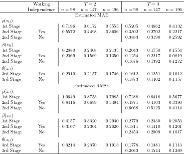
Table 2. Simulation Results for the Estimator Using Linear Moments Only
Working T = 2 T = 3
Independence n= 98 n= 147 n= 196 n= 98 n= 147 n= 196 Estimated MAE
ρ(zit)
1st Stage 0.7196 0.6172 0.5555 0.5205 0.4662 0.4132 2nd Stage Yes 0.5572 0.4498 0.3606 0.3302 0.2702 0.2217 2nd Stage No 0.3883 0.3190 0.2592
β(zit)
1st Stage 0.2880 0.2408 0.2135 0.2043 0.1750 0.1554 2nd Stage Yes 0.2069 0.1569 0.1350 0.1254 0.2217 0.0819 2nd Stage No 0.1676 0.1392 0.1272
θ(zit)
3rd Stage Yes 0.2910 0.2157 0.1746 0.1612 0.1251 0.1012 3rd Stage No 0.1873 0.1402 0.1157
Estimated RMSE ρ(zit)
1st Stage 1.0649 0.8753 0.7985 0.7288 0.6418 0.5677 2nd Stage Yes 0.8416 0.6699 0.5494 0.4871 0.4103 0.3380 2nd Stage No 0.6068 0.5125 0.4114
β(zit)
1st Stage 0.4157 0.3320 0.2930 0.2779 0.2330 0.2053 2nd Stage Yes 0.3107 0.2304 0.2020 0.1811 0.1410 0.1201 2nd Stage No 0.2453 0.2009 0.1817
θ(zit)
3rd Stage Yes 0.3214 0.2370 0.1913 0.1778 0.1381 0.1113 3rd Stage No 0.2063 0.1544 0.1269
when constructing the matrix of linear instruments Q, andPn,l =IT−1⊗Wl0−n−1tr
Wl 0 In forl= 1,2 for quadratic moments. For the second-stage estimation, Qb(z) and Pbn are constructed using first-stage estimates ofρ(zit) and β(zit) as described in Section 3.1.
For each sample size, we simulate the model 500 times. For each simulation, we compute the mean absolute error (MAE) and the root mean squared error (RMSE) for each functional coefficient. Reported are their averages computed over 500 simulations. We report the results for both the first-and second-stage nonparametric GMM estimators fitted using two sets of orthogonality conditions:
(i) linear and quadratic moments (Table 1) and (ii) linear moments only (Table 2). Also, for
T = 3, we estimate the second-stage model twice: (i) accounting for “random effects” in ∆uit induced by first-differencing as outlined in Section 3.1 and(ii) ignoring them by applying the local Taylor approximation directly to (3.8) [as opposed to (3.11)]. In the second columns in both tables, “Yes” corresponds to case (ii) with the “working independence” assumption imposed, while “No” corresponds to case (i).
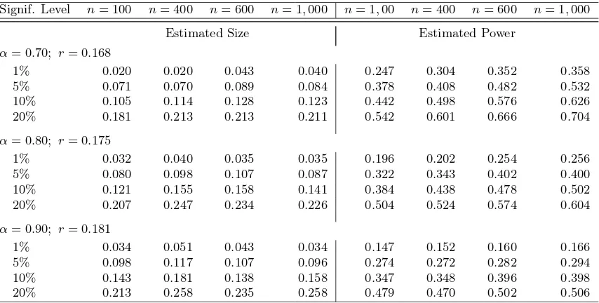
Table 3. Simulations Results for the Spatial Endogeneity Test
Signif. Level n= 100 n= 400 n= 600 n= 1,000 n= 1,00 n= 400 n= 600 n= 1,000
Estimated Size Estimated Power α= 0.70; r= 0.168
1% 0.020 0.020 0.043 0.040 0.247 0.304 0.352 0.358 5% 0.071 0.070 0.089 0.084 0.378 0.408 0.482 0.532 10% 0.105 0.114 0.128 0.123 0.442 0.498 0.576 0.626 20% 0.181 0.213 0.213 0.211 0.542 0.601 0.666 0.704
α= 0.80; r= 0.175
1% 0.032 0.040 0.035 0.035 0.196 0.202 0.254 0.256 5% 0.080 0.098 0.107 0.087 0.322 0.343 0.402 0.400 10% 0.121 0.155 0.158 0.141 0.384 0.438 0.478 0.502 20% 0.207 0.247 0.234 0.226 0.504 0.524 0.574 0.604
α= 0.90; r= 0.181
1% 0.034 0.051 0.043 0.034 0.147 0.152 0.160 0.166 5% 0.098 0.117 0.107 0.096 0.274 0.272 0.282 0.294 10% 0.143 0.181 0.138 0.158 0.347 0.348 0.396 0.398 20% 0.213 0.258 0.235 0.258 0.479 0.470 0.502 0.506
accounts for random effects with its pooled local linear alternative, we observe that the estimation of β(·) benefits significantly from the “working independence” assumption, at least in our current data generating design.
Tables 1 and 2 also report the results for the third-stage sieve estimator of θ(·). We use cubic B-splines to approximate the unknown functional coefficient. For simplicity, we set Ln= 3 in our experiments for all three differentn’s since the range of the sample size is not that large. Consistent with our theory, the sieve estimator of θ(·) becomes more stable as the sample size grows.
Overall, simulation experiments lend support to asymptotic results for our proposed estimators.
7.2 Spatial Endogeneity Test
We next examine the small sample performance of our proposed residual-based test statistic for spatial endogeneity. To assess the size and power of our test statisticJn, we consider the following two experimental designs for the data-generating process given in (7.1), wherezit,xit,gi,uit,µi and the functional coefficients θ(·) andβ(·) are generated exactly as in Section 7.1. Following Kelejian & Prucha (1999) and Jin & Lee (2015), we choose a circular “1 ahead and 1 behind” structure of W0 ={wij}ni,j=1, where a given spatial unit is related to one neighbor immediately ahead and one neighbor immediately behind it in a row. Each of these two neighbors are assigned an equal non-zero weight of 0.5. We then specify the spatial lag functional parameterρ(·) as follows:
(i) No spatial dependence: ρ(zit) = 0 for allzit;
(ii) Spatial autoregression: ρ(zit) = 0.5 + 0.4 exp(−2zit).
We consider samples with n={100, 400, 600, 1,000} andT = 3. For eachn, we simulate the model 500 times. We seteh0 = 1.06σbz(n(T−1))−0.20,eh= 1.06bσz(n(T−1))−0.45,h0 = 1.06σbz(n(T− 1))−α and h = 1.06σb
Table 3 reports the estimated size under design (i) and power under design (ii) of our test statistic which are computed as rejection frequencies out of 500 simulations. Here, we use (asymptotic) standard normal critical values. We find that out test statistic Jn exhibits good power which increases with the sample size as anticipated, regardless of the choice of bandwidths. Also, the power is significantly better when we under-smooth in both stages under H1. The size of the test also seems to be sensitive to the degree of smoothing under the alternative with the better results reported for the case when α = 0.70 and r = 0.168, which imply stronger under-smoothing under
H1. Overall, the estimated size tends to be greater than the nominal level, which is quite expected given that we use asymptotic critical values and kernel-based nonparametric tests are known to be prone to finite-sample size distortions. In empirical applications, we certainly recommend using the bootstrap method.
8
Conclusion
This paper proposes an innovative way of estimating a functional-coefficient spatial autoregressive panel data model with unobserved individual fixed effects which can accommodate (multiple) time-invariant regressors in the model. The methodology we propose removes unobserved fixed effects from the model via the first-difference transformation. The estimation of the transformed non-parametric additive model however does not require the use of backfitting or marginal integration techniques. We derive the consistency and asymptotic normality results for the proposed kernel and sieve estimators. We also construct a consistent nonparametric test statistic to test for spatial endogeneity in the data. A small Monte Carlo study shows that both our proposed estimators and the test statistic exhibit good finite-sample performance.
Appendix. Brief Mathematical Proofs
Proof of Theorem 1. Denoteϑn=ζn
h b˙
θ(z)′−θ˙(z)′ γb(z)′−γ(z)′
i′
,△y∗
it=△yit−gi′θ˙(z)−
ξ′m′
itγ(z) and εit(ϑ) = △yit∗ −ζn−1
g′
i,ξ′m′it
ϑ, where {ζn} is a sequence of positive constants such that 0< C1 <kϑnk< C2<∞for all nand T. We then rewrite (3.6) as
gn(ϑ) =
ε(ϑ)′Kh(z)Pn,1Kh(z)ε(ϑ) ..
.
ε(ϑ)′Kh(z)Pn,LKh(z)ε(ϑ)
Q′K
h(z)ε(ϑ)
, (A.1)
whereε(ϑ) is an [n(T −1)]×1 vector stacking up{εit(ϑ)} in the ascending order of indext first then indexi, and obtain the following:
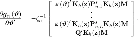
∂gn(ϑ)
∂ϑ′ =−ζ
−1 n
ε(ϑ)′Kh(z)Psn,1Kh(z)M ..
.
ε(ϑ)′Kh(z)Psn,LKh(z)M
Q′K
h(z)M
.
inϑ∈S, a compact subset of R2(dx+1)+dg. Sinceϑ
nminimizes Λn(ϑ) =gn(ϑ)′gn(ϑ), we have
02(dx+1)+dg = ∂gn(ϑn)
′
∂ϑ gn(ϑn) =
∂gn(ϑn)′
∂ϑ
gn(0) +
∂gnϑen
∂ϑ′ ϑn
,
whereϑen lies betweenϑn and 02(dx+1)+dg, and hence:
ϑn=−
∂gn(ϑn)′
∂ϑ
∂gnϑen
∂ϑ′
−1
∂gn(ϑn)′
∂ϑ gn(0) .
Specifically, denoting Ξh(z)≡Kh(z)QQ′Kh(z), we have
An(z) = −
∂gn(ϑn)′
∂ϑ gn(0)
= 1
2ζn L
X
l=1
M′Kh(z)Pn,ls Kh(z)ε(ϑn) ∆y∗′Kh(z)Pn,ls Kh(z)∆y∗+ 1
ζn
M′Ξh(z)∆y∗
and
Bn(z) =
∂gn(ϑn)′
∂ϑ
∂gnϑen
∂ϑ′
= 1
ζ2 n
L
X
l=1
ε(ϑn)′Kh(z)Psn,lKh(z)M ′ε
e
ϑn
′
Kh(z)Psn,lKh(z)M+ 1
ζ2 n
M′Ξh(z)M.
For each (i, t), we have△y∗
it=△uit+cit(z), wherecit(z) =g′i[θ(zit)−θ(z1)]−gi′[θ(zi,t−1)−θ(z2)] +m′it[γ(zit)−γ(z1)]−m′i,t−1[γ(zi,t−1)−γ(z2)]. Stacking up{cit(z)}in the ascending order of in-dextfirst then indexigives an [n(T−1)]×1 vectorC(z). We also denote Γ1,l =△u′Kh(z)Pn,ls Kh(z)C(z), Γ2,l =C(z)′Kh(z)Psn,lKh(z)C(z), Γ3,l =△u′Kh(z)Psn,lKh(z)∆u, Ψ1,l =△u′Kh(z)Psn,lKh(z)M, Ψ2,l =C(z)′Kh(z)Psn,lKh(z)M and Ψ3,l =M′Kh(z)Pn,ls Kh(z)M forl= 1, . . . , L. Then, we have
An(z) =An1(z) +An2(z)−An3(z) with
An1(z) = 1 2ζn
L
X
l=1
(2Γ1,l+ Γ2,l+ Γ3,l) (Ψ1,l+ Ψ2,l)′+ 1
ζn
M′Ξh(z)C(z),
An2(z) = 1
ζn
M′Ξh(z)∆u,
An3(z) = 1 2ζ2
n L
X
l=1
(2Γ1,l+ Γ2,l+ Γ3,l) Ψ3,lϑn
and
Bn(z) = 1
ζ2 n
L
X
l=1
Ψ1,l+ Ψ2,l− 1
ζn
ϑ′nΨ3,l
′
Ψ1,l+ Ψ2,l− 1
ζn
e
θ′nΨ3,l
+ 1
ζ2 n
M′Ξh(z)M.
By Lemmas 1–3 below, we have