Local Explosion Modelling by Noncausal Process

Munich Personal RePEc Archive

Local Explosion Modelling by Noncausal

Process

Gouriéroux, Christian and Zakoian, Jean-Michel

CREST and University of Toronto, CREST and Université de Lille

5 May 2016

Online at

https://mpra.ub.uni-muenchen.de/71105/

Local Explosion Modelling by Noncausal Process

Christian Gouriéroux

CREST and University of Toronto

Jean-Michel Zakoïan

CREST and Université de Lille

May 5, 2016

Abstract. The noncausal autoregressive process with heavy-tailed errors possesses a

non-linear causal dynamics, which allows for local explosion or asymmetric cycles often observed

in economic and financial time series. It provides a new model for multiple local explosions in

a strictly stationary framework. The causal predictive distribution displays surprising features,

such as the existence of higher moments than for the marginal distribution, or the presence

of a unit root in the Cauchy case. Aggregating such models can yield complex dynamics with

local and global explosion as well as variation in the rate of explosion. The asymptotic behavior

of a vector of sample autocorrelations is studied in a semi-parametric noncausal AR(1)

frame-work with Pareto-like tails, and diagnostic tests are proposed. Empirical results based on the

Nasdaq composite price index are provided.

Keywords: Causal innovation, Explosive bubble, Heavy-tailed errors, Noncausal process,

Sta-ble process.

Address for correspondence: Jean-Michel Zakoïan, CREST, 15 Boulevard Gabriel Péri,

92245 Malakoff cedex. Email: [email protected]

1. Introduction

A number of economic and financial time series possess nonlinear dynamic features such

as asymmetric cycles [Ramsey and Rothman (1996)] or speculative bubbles.1

It has been

noted that the mixed causal and noncausal linear autoregressive (AR) processes often

pro-vide a better fit to such time series than the standard causal autoregressive moving-average

(ARMA) processes [see e.g. Lanne et al. (2012), Lanne, Saikkonen (2011), Davis, Song

(2012), Chen et al. (2012)]. The traditional Box-Jenkins methodology based on Gaussian

linear processes were found insufficient to capture such features. Indeed, Gaussian AR

processes are the only processes with both causal and noncausal strong linear AR

repre-sentations2

[see Cheng (1992), Breidt, Davis (1992)]. In contrast, a non-Gaussian linear

noncausal process admits a nonlinear dynamics in direct time, which may produce local

explosion whenever the errors distribution has fat tails.

The aim of this paper is to analyze the dynamic properties of heavy-tailed noncausal

linear AR(1) processes that do not admit a causal linear AR representation, and to

under-stand their potential usefulness in applications. In particular, it provides a new model for

multiple local explosions in a strictly stationary framework. The transition distribution in

direct time displays surprising features, such as the existence of higher moments than for

the marginal distribution, or the presence of a unit root in the Cauchy case. We will also

show how such processes can be combined to disentangle local and global explosive patterns

and for modeling recursive explosions with different rates.

The paper is organized as follows. Section 2 reviews the main properties of strong

linear processes in the presence of heavy-tailed errors. In particular, we explain how local

explosion can arise when the linear process has a noncausal component and heavy-tailed

errors. Section 3 considers noncausal AR(1) processes with stable errors. We characterize

their stationary distribution and the existence of conditional moments. In the cases of the

noncausal AR(1) models with Cauchy and Lévy errors, we derive the closed form formula of

the conditional density in direct time. These results are used to obtain semi-strong causal

representations of the process. Aggregation of noncausal AR(1) processes is studied in

Section 4. Such aggregated processes are used to model local explosions with different rates

of explosion. We explain how to identify the different components and to disentangle local

admit a multiplicity of solutions, some of them featuring local explosions followed by a crash. Such phenomena are called explosive or speculative bubbles by other authors [see e.g. Diba and Grossman (1988), Evans (1991)]. In this article we only consider the second concept, interpreting bubbles in a statistical sense, as local explosive behaviours.

explosion components and global trend. In Section 5 we derive the asymptotic properties

of the sample autocorrelations for the noncausal Cauchy AR process. Next we explain

why the standard unit-root tests based on the detection of global stochastic trends can be

misleading when looking for local explosions. Finally, we study diagnostic tools.

Monte-Carlo experiments are presented in Section 6. An application on real data is proposed in

Section 7. Section 8 concludes. Proofs of the propositions and complementary results are

gathered in an appendix.

2. Strong linear processes

We consider a strong linear process(Yt), that is a two-sided moving average process:

Yt= ∞ X

h=−∞

ahεt−h, (2.1)

where (εt) is a sequence of independent and identically distributed (i.i.d.) real random

variables,(ah)is a sequence of real coefficients, satisfying for somes∈(0,1),

E_|εt|s<∞ and ∞ X

h=−∞

|ah|s<∞. (2.2)

It follows from Proposition 13.3.1 in Brockwell and Davis (1991) that the process (Yt)in

(2.1) is well defined. Whenah = 0 for allh < 0, the process (Yt)is called purely causal

(with respect to (εt)); when ah = 0 for all h > 0, (Yt) is called purely noncausal. The

uniqueness of the MA representation in (2.1) with heavy-tailed errors was recently studied

by Gouriéroux and Zakoian (2015).

The trajectory of a strong linear process can be considered as a stochastic combination

of baseline deterministic functions.

i) Let us consider a strong purely causal (or backward looking) process. This process can

be written as: Yt= +∞ X

τ=−∞

ετ1lτ≤tat−τ.Thus, the path of process(Yt)is a combination of

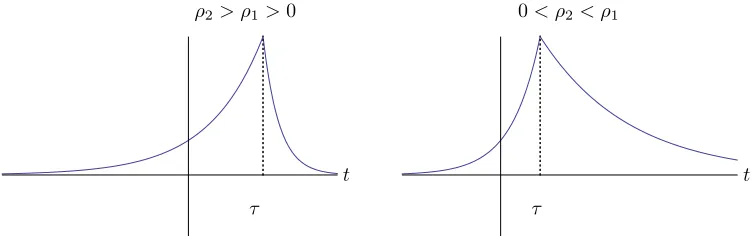
baseline paths Zτ(t) = 1lτ≤tat−τ, with stochastic i.i.d. coefficientsετ. Figure 1, left panel,

provides an illustration for a causal AR(1) process, Yt = ρYt−1+εt with |ρ| < 1 (thus

ah=ρh for h≥0). The baseline path shows an upward jump followed by an exponential

decrease.

ii) If now(Yt)is a strong purely noncausal (or forward looking) process, we have:

Yt = +∞ X

τ=−∞

1lτ≤tρt−τ 1lτ≥tρτ−t

t t

τ τ

Figure 1.The baseline paths for causal and noncausal AR processes

ρ2> ρ1>0 0< ρ2< ρ1

t t

τ τ

Figure 2.The baseline paths1lτ≤tρ1t−τ+ 1lτ >tρτ2−tfor mixed AR(2) processes

The path of process(Yt)is now a combination of the baseline pathsZτ(t) = 1lτ≥taτ−t, with

stochastic i.i.d. coefficients ετ. Figure 1, right panel, illustrates this baseline path for a

noncausal AR(1) process,Yt =ρYt+1+εt with |ρ| <1 (thusa−h = ρh for h≥ 0). The

baseline path features an explosive growth followed by a vertical downturn att=τ.

iii) Let us finally consider a mixed (causal and noncausal) process. The path of (Yt)is a

combination of the baseline pathsZτ(t) = 1lτ <tat−τ+ 1lτ≥taτ−t, with stochastic i.i.d.

co-efficients ετ. For instance, if the model is the mixed AR(2): (1−ρ1B)(1−ρ2F)Yt =

εt, |ρ1|<1,|ρ2|<1,where B andF are the backward and forward operators,

respec-tively, we getZτ(t) = (1−ρ1ρ2)−1 1lτ <tρt1−τ+ 1 + 1lτ >tρτ2−t

. The baseline path features

The noncausal MA(_∞) representation (2.3) helps understanding the formation of

bub-bles in the dynamics of noncausal processes. First note that the presence of potentially fat

tailed error distributions is likely to produce extreme values of any sign over a finite time

period. Now suppose that a very large, say positive, valueετoccurs at timeτ. According to

(2.3) if, for simplicity, the sequence(ah)is strictly decreasing, fort≤τ the weight of that

extreme value increases ast approaches τ. This explains the growth phase of the bubble.

Att=τ+ 1, the extreme value cancels out from the sum and the bubble bursts.

There are two types of asymmetries in the shape of a bubble. Longitudinal

asymme-tries arise in calendar time when the growth and downturn periods have different lengths,

as illustrated in Figure 2. Transversal asymmetries arise when the curvature (resp. the

magnitude) at a peak and at a trough are different due to the coefficients of the MA(∞)

representation (resp. to the asymmetric tails of the error distribution).

3. The noncausal stable linear AR(1) process

In this section, we consider noncausal AR(1) processes with stable distributed errors. Let

X_{∼ S}(α, β, σ, µ)denote a variable following anα-stable distribution, whereα_∈(0,2]is the

index of stability,β∈[−1,1]is an asymmetry parameter,σ∈(0,∞)is a scale parameter,

andµ∈Ris a location parameter.

In general, the probability density function (pdf) of a stable distribution is not known

explicitly, but its characteristic functionψ(s) =E(eisX_{)has the closed form:}

logψ(s) =₋σα_|s_|αn1₋iβ(signs) tanπα 2

o +iµs,

ifα₆= 1, and

logψ(s) =₋σ_|s_|

1 +iβ(signs)2 πlog|s|

+iµs,

ifα= 1, where sign(x) denotes the sign of a real numberx. The stable distribution with

β = 0 and exponentα= 2 (resp. α= 1) is the Gaussian distribution N(µ, σ2_{) (resp. the}

Cauchy distribution_C(µ, σ)whose pdf is σ

π{(x−µ)2_+σ2_}) . The coefficient αdetermines the

tails of the distribution ofX ∼S(α, β, σ, µ) in the sense that, whenα <2,

E_|X_|p_<

∞ if and only if p < α. (3.1)

3.1. The process

Let us consider the forward looking AR process:

Yt=ρYt+1+εt, |ρ|<1, εt∼ S(α, β, σ,0), (3.2)

with i.i.d. backward "innovations"εt.3 In view of (3.1) and condition (2.2), the strictly

stationary solution of equation (3.2) is given by:

Yt= ∞ X

h=0

ρhεt+h. (3.3)

The stationary distribution of(Yt)is provided in the next proposition.

Proposition 3.1. The noncausal stable linear AR(1) process (3.2) has a stable

station-ary distribution given by:

Yt ∼ S

α, β, σ

(1_{− |}ρ_|α₎1/α,0

, if α₆= 1, ρ_≥0,

Yt ∼ S

α, β1− |ρ| α

1 +_|ρ_|α, σ

(1_{− |}ρ_|α₎1/α,0

, if α6= 1, ρ≤0,

Yt ∼ S

1, β1− |ρ| 1₋ρ,

σ

1_{− |}ρ_|,−βσ 2 π

ρlog|ρ|

(1₋ρ)2

, if α= 1.

In particular, the stationary distribution of the noncausal Cauchy linear AR(1) process

(α = 1, β = 0) is the Cauchy distribution _C0, σ 1−|ρ|

. When ρ _≥ 0, the asymmetry

parameter of Yt is that of the innovation ǫt; when ρ < 0, the sign of the asymmetry is

unchanged, but the asymmetry coefficient is smaller. Finally, when α = 1 and β 6= 0, a

location parameter appears in the distribution ofYt.

Now, let us consider the process in direct time. While for α <2 the backward stable

transition pdf f(Yt|Yt+1) features fat tails, so that the p-th conditional moments do not

exist forp_≥α, the next proposition shows that the forward transition pdf at any horizon

admits Pareto tails with tail parameter equal to 2α+ 1, whenever ρ ₆= 0. In the causal

AR(1) framework, similar results were obtained by Cambanis and Fakhre-Zakeri (Theorem

3, 1994) for the one-step predictor (h= 1) with time reversed.

Proposition 3.2. The noncausal stable linear AR(1) process (3.2) is an homogeneous

Markov process. Letα <2. For anyh_≥0, if_|β_{| 6}= 1andρ₆= 0, or if_|β_|= 1andρh+1_<0,

we have

E(_|Yt+h|p|Yt−1)<∞, a.s., if and only if −1< p <2α+ 1. (3.4)

3_{Strictly speaking, innovations are not defined whenα}

≤1because E(Yt |Yt+1)does not exist

If_|β_|= 1 andρh+1_{>0, thenE(}

|Yt+h|p|Yt−1)<∞, a.s. for allp >−1.

In particular, the forward conditional expectation E(Yt+h | Yt−1) always exists, whereas

the unconditional and backward conditional expectations exist only whenα >1.The next

result gives a closed-form expression of the conditional expectation for symmetric stable

distributions.

Proposition 3.3. Forρ6= 0 andβ= 0, we have:

E(Yt+h |Yt−1) = sign(ρ)|ρ|(h+1)(α−1)Yt−1, ∀h≥0.

In particular, for Cauchy processes (α= 1), whenρ₆= 0 we have:

E(Yt+h|Yt−1) = sign(ρ)Yt−1, ∀h≥0.

This result is unexpected. Indeed, in the L2 _{framework, if (X}

t) is a stationary strong noncausal AR(1): Xt=ρXt+1+Wt, |ρ|<1, Wtiid∼(0, σ2),then(Xt)can be expressed

as aweak causalAR(1) with the same AR coefficient: Xt=ρXt−1+Wt∗,where(Wt∗)is a

weak white noise with varianceσ2_{(see e.g. Brockwell and Davis (1991), Proposition 4.4.2).}

It follows that if E(Xt | Xt−1) is linear in Xt−1, we must have E(Xt | Xt−1) = ρXt−1.

In contrast, Proposition 3.3 shows that the first-order prediction of Yt is E(Yt | Yt−1) =

|ρ|α−1_Y

t−16=ρYt−1. The Cauchy process, forα= 1, is even more intriguing as it has a unit

root whenρ >0, although the process is stationary.

Remark 3.1 (Stable AR(1) process with drift). The introduction of a location parameter in the stable distribution of the innovations (ǫ∗

t) is tantamount to adding an intercept to Model (3.2). The noncausal stable linear AR process with driftµwrites

Zt=µ+ρ∗Zt+1+ε∗t, |ρ∗|<1. (3.5)

Studying the solutions to this model is straightforward, noting that there is a one-to-one

relation between the solutions(Yt)of Model (3.2) and (Zt)of model (3.5) via the relation

Yt=Zt−₁₋µ_ρ∗.It thus follows from Proposition 3.5 that, forρ∗6= 0, we have, forh≥0:

E(Zt+h|Zt−1) =|ρ∗|(h+1)(α−1)Zt−1+

µ 1−ρ∗

1_{− |}ρ∗_|(h+1)(α−1)_.

Interestingly, the adjunction of a constant does not remove the martingale property in the

Cauchy case (α= 1 andρ∗_>0).

3.2. Causal predictive distributions in the Cauchy and Lévy cases

The predictive distributions of the process(Yt)(and the causal first and second-order

mo-ments when they exist) generally do not admit closed form expressions. Two exceptions are

the noncausal AR(1) processes with Cauchy and Lévy backward innovations, obtained for

(α, β) = (1,0)and(α, β) = (1/2,1), respectively.

3.2.1. Noncausal Cauchy linear AR(1) process

The following result gives the Markov transition of the process(Yt)in direct time.

Proposition 3.4. The causal transition pdf of the noncausal Cauchy linear AR(1)

pro-cess at horizon his given by:

fh(Yt|Yt−h) = 1 πσh

1

1 + (Yt−h−ρhYt)2/σ2h

σ2+ (1− |ρ|)2Yt2−h σ2_{+ (1− |ρ|)}2_Y2

t

, where σh=σ 1_{− |}ρ_|h

1− |ρ| .

Therefore, the Pareto tail index of the predictive density is equal to 4, at any prediction

horizon. This is only in the limiting case h = _∞ that we observe a discontinuity in the

value of the tail index, that is, for the stationary distribution. Straightforward calculation

shows that the conditional densityfh(· |Yt−h)is unimodal, for any value ofYt−h.

Proposition 3.4 allows to obtain the causal conditional cdf of the noncausal Cauchy

process (see Appendix B). The process also admits a strong causal nonlinear autoregressive

representation which is derived in Appendix C.

The first and second-order causal conditional moments of the process exist by

Proposi-tion 3.4. The condiProposi-tional mean was derived in ProposiProposi-tion 3.3. We now give a closed-form

expression of the conditional second-order moment for the noncausal Cauchy process.

Proposition 3.5. Forρ6= 0, whenα= 1andβ = 0in Model (3.2), we have:

E(Yt|Yt−1) = sign(ρ)Yt−1, E(Yt2|Yt−1) =

1

|ρ|Y

2 t−1+

σ2

|ρ|(1− |ρ|).

Despite the nonlinear causal autoregression, both processes (Yt) and (Yt2) admit a

semi-strong linear causal representation, that is, with linear causal innovationsYt−E(Yt|Yt−1)

andY2

t −E(Yt2|Yt−1), respectively, that are martingale difference sequences, but not i.i.d.

In fact, (Yt)has a semi-strong AR(1) representation of the form:

Yt = sign(ρ)Yt−1+σtηt, σ2t = ₁

|ρ|−1

Yt2−1+

σ2

|ρ|(1− |ρ|), (3.6)

where E(ηt| Yt−1) = 0, E(η2t |Yt−1) = 1. Whenρ > 0, the process (Yt)is a

GARCH-type effects, which increase whenρapproaches 0, but vanish when_|ρ_|increases to

1. In view of (3.6),(Yt)might be called a double semi-strong AR(1) process (see Ling and

Li (2008)). However, the innovationsηt are not independent. Indeed, by Proposition 3.4

forh= 1, the conditional density ofηtdepends on the past: withYtgiven by (3.6),

fη(ηt|Yt−1) =

1 p

|ρ_|(1_{− |}ρ_|)π

σ_{σ2_{+ (1}

− |ρ_|)2_Y2

t−1}3/2

{σ2_{+ (Y}

t−1−ρYt)2}{σ2+ (1− |ρ|)2Yt2} .

The recursive equations (3.6) associated with the first and second-order conditional causal

moments seem explosive: the AR coefficient on the squareY2

t is1/|ρ|>1and the coefficient ofYt−1 in the expression ofE(Yt|Yt−1)leads to a unit root phenomenon, ifρ >0, and to

a periodicity with period 2, ifρ <0. This is not surprising since the unconditional first and

second-order moments do not exist. However, the infinite moments of the unconditional

distribution do not have the same implications on the process in reverse time. Indeed, in

reverse time the process does not explose, since _|ρ_| < 1, and infinite moments are just a

consequence of the fat tail of the backward innovations. Similar formulas can be derived at

any prediction horizonh >0 withρreplaced byρh _andσbyσ

h,respectively.

3.2.2. Noncausal Lévy Autoregressive Process

Let us now consider Model (3.2) under the assumption that εt ∼ S(1/2,1,1,0), that is

whenεtfollows a Lévy (µ, c) distribution with parametersµ= 0, c= 1. This means thatεt

only takes positive values, which is appropriate for modelling (positive) prices or nominal

interest rates. More precisely, the density ofεtis given by:

fε(x) = 1

√

2π 1 x3/2exp

−1

2x

Ix>0. (3.7)

Let us assume ρ > 0 to ensure the positivity of Yt. By Proposition 3.1, the stationary

distribution ofYtis also a Lévy distribution, with parametersµ= 0, c= 1/(1−√ρ)2.Thus,

the stationary density of the noncausal Lévy linear AR process is:

f(y) = √1

2π 1 1₋√ρ

1 y3/2exp

−1

2y 1 (1₋√ρ)2

Iy>0. (3.8)

Proposition 3.6. The causal transition pdf of the noncausal Lévy linear AR process, withρ >0, is given by:

f(Yt|Yt−1) = 1

√

2π

Yt−1

Yt(Yt−1−ρYt) 3/2

exp

−(Yt−1−√ρYt)

2Yt−1Yt(1−√ρ)2(Yt−1−ρYt)

0 50 100 150 200

0

100

200

300

0 50 100 150 200

0

20

40

60

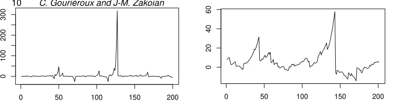
Figure 3. Simulations of Model (3.2) withα= 1, β = 0,σ = 0.5andρ = 0.5(left panel),ρ= 0.9

(right panel).

The support of the causal transition pdf is bounded from above. For this reason, the

maximum rate of explosion of a bubble is 1/ρ. It is also worth noting that the moments

ofYtconditional onYt−1exist at any order (which also follows from Proposition 3.2 in the

caseβ = 1andρ >0), whereas the unconditional expectation of Yt does not exist.

By Proposition 3.3, the process has a semi-strong AR(1) causal representation: Yt= 1

√_ρYt−1+vt,whereE(vt|Yt−1) = 0. The bubble phenomenon can be more prominent than

with Cauchy distributed errors, especially whenρis close to zero.

3.3. Locally explosive phenomena

In Section 2 we have shown that the path of a noncausal linear AR process is a combination

of right-censored increasing exponential curves (ifρ >0) with i.i.d. stochastic coefficients.

When the error distribution has fat tails, an extreme value from the right tail creates a jump

of Yt preceded by a local upward trend toward that extreme value. Conversely, an error

from the left tail will create a symmetric pattern, able to represent a deflationary spiral.

Depending on the purpose, the noncausal model can be adapted to only one type of locally

explosive phenomenon, bubble or deflationary spiral, by choosing an error distribution on

R+with a fat right tail, or onR− with a fat left tail.

We provide in Figure 3 the simulated paths of the noncausal Cauchy process based

on the forward autoregression (3.2), where theεt are drawn independently in the Cauchy

distribution (withσ= 1) andρ= 0.5 (left panel) orρ= 0.9 (right panel). Forρ= 0.9, we

clearly observe the bubble phenomenon at regular intervals. Note that the bubble collapse

can be sudden, i.e. a crash within single period, or it can take place gradually.

The heavy-tailed noncausal AR models can represent multiple local explosions and offer the

noncausal innovation takes an extreme value, and the date at which that extreme value is

reached is the date of bubble collapse. Therefore, it is possible to predict the date of a bubble

collapse by considering the extreme behaviour of noncausal innovationsεt.4 At time t, we

can compute the probability of a bubble collapse att+hasP(Yt+h−ρYt+h+1> c|Yt), for

some extreme critical levelc. By updating these probabilities and following their evolution,

we obtain a tool for early warning of the bubble collapse. Thus, contrary to a belief common

to economists (see e.g. Cooper (2008)), it seems possible to detect a bubble in its inflationary

phase, and to predict the future bubbles (see Phillips et al. (2015) for a similar remark).

4. Aggregation of noncausal processes

4.1. Aggregation of a continuum of noncausal Cauchy AR(1)

Noncausal AR(1) processes with stable distributions can generate a series of local

explo-sions, but only with the same (stochastic) rate of increase determined by the coefficientρ.

Aggregation of such basic processes allows us to get bubbles with different rates of increase.

For simplicity, we focus on basic Cauchy AR(1) processes in this section.

Let us first consider an aggregate process from a finite set of noncausal Cauchy AR(1)

processes. The process is defined by

Yt=c

J X

j=1

πjYj,t, with Yj,t=ρjYj,t+1+εj,t, |ρj|<1, j= 1, . . . , J, (4.1)

where (εj,t)j=1,...,J is a family of i.i.d. standard Cauchy white noises, c > 0, πj ≥0 and PJ

j=1πj = 1. By construction, this process can generate successive bubbles, with rates

of increases 1/ρj (if ρj > 0) and occurrences governed by the weights πj. However, the

aggregation destroys the Markov property of the noncausal aggregate process in reverse

time.

The aggregation can be extended to a continuum of values of parameter ρ, with a

probability distributionπon(₋1,1)(which can be either continuous or discrete). Let

Yt:=Yt(c, π) =c Z

(−1,1)

Yρ,tdπ(ρ), (4.2)

where Yρ,t =ρYρ,t+1+ερ,t, |ρ| < 1, c > 0, and (ερ,t) are i.i.d. standard Cauchy white

noises. Let us denoteEπ(f) =Rf(ρ)dπ(ρ)for any functionf : (−1,1)7→Rsuch that the

integral exists. The following proposition gives a sufficient condition for the existence of

processYt.

Proposition 4.1. Assume that, for somes∈(0,1), ∞

X

i=0

Eπ(|ρ|i|) s

<_∞. (4.3)

Then,Yt is well defined and we have:

Yt=

X

i≥0

Z ρi_ε

ρ,t+idπ(ρ). (4.4)

Moreover, the process(_Yt)t≥0 is strictly stationary and ergodic, andYt follows the Cauchy

distribution with scale parametercEπ n

1 1−|ρ|

o .

Example 4.1 (Discrete measure). Suppose that the support of probability measure π is _{ρj}j∈N, where the ρ_j’s belong to (−1,1) and are ranked in increasing order. Let

πj =π({ρj})(withπj>0andPj≥0πj= 1). Then, the condition in (4.3) becomes

∞ X i=0    X

j≥0

|ρj|iπj

   s

<_∞. (4.5)

Using the elementary inequality (x+y)s _{≤ x}s_+ys_{, for x, y ≥ 0 and s ∈ (0,1), we get}

a sufficient condition for strict stationarity: P_j≥0 π s j

1−|ρj|s <∞, and a necessary condition for the existence of the sum in (4.5) is: Eπ

1 1−|ρ|

= Pj≥0 πj

1−|ρj| < ∞. For instance if πj = ˜πj forj >0 and |ρj|= 1−ρ˜j, for someπ,˜ ρ˜∈(0,1), a necessary condition for strict

stationarity of(Yt)isπ <˜ ρ˜.

The distribution of the strictly stationary aggregated process is characterized by its

characteristic functionΨ(u0, . . . , uk) =E[exp{i(Pkℓ=0uℓYt+ℓ)}], for(u0, . . . , uk)∈Rk+1.

Proposition 4.2. Assume that (4.3) holds and, for anyt∈Z, assume that the process

{ερ,t,(ρ, t)∈(−1,1)×Z+} is independent. We have, for (u0, . . . , uk)∈Rk+1,

Ψ(u0, . . . , uk) = exp   −cEπ

 

k−1

X h=0 h X ℓ=0

ρh−ℓuℓ +

Pkℓ=0ρk−ℓuℓ 1_{− |}ρ_|

 

  .

Thus, the linear combination Pk_ℓ=0uℓYt+ℓ follows a Cauchy distribution, with scale

pa-rameter equal to the expectation in the brackets. The joint distribution of (_Yt,Yt+k) is

characterized below.

Corollary 4.1. Under the assumptions of Proposition 4.2, we have

E[exp_{i(u0Yt+ukYt+k)}] = exp

−cEπ

1

1_{− |}ρ_| |u0|(1− |ρ| k_{) +}

|ρku0+uk|

4.2. Identification and estimation of the explosive patterns

Let us now show that the parameters characterizing the local explosive patterns are

iden-tifiable from the bivariate distribution of(Yt,Yt+1).

4.2.1. Identification

From Corollary 4.1, it follows that

˜

Ψ(u) := logE[exp_{i(_Yt+uYt+1)}] =−cEπ

1 + |ρ+u| 1− |ρ|

. (4.6)

The proposition below shows how to derive the local explosion parameterscandπfrom the

joint characteristic functionΨ˜. LetΨ˜(2)_{(u) =} ∂2_{Ψ(˜ u)}

∂u2 .

Proposition 4.3. Assume that the measureπadmits a density,dπ(ρ) =π(ρ)dρ. Then,

under (4.3), the parametersc, πare identifiable from the joint distribution of(Yt,Yt+1). We

have, forρ_∈(₋1,1),

π(ρ) = (1− |ρ|) ˜Ψ

(2)_(−ρ)

R1

−1(1− |u|) ˜Ψ(2)(−u)du

, c=−1₂

Z 1

−1

(1− |u|) ˜Ψ(2)(−u)du.

4.2.2. Estimation of the local explosion structure

The relations in Proposition 4.3 can be used to estimate the density π and the constant

c from observations _Y1, . . . ,Yn. First note that, because the distribution of (Yt,Yt+1)is

symmetric, we haveΨ(u) = log˜ E[cos(_Yt+uYt+1)]. It follows that

˜

Ψ(2)(u) =₋E[Y

2

t+1cos(Yt+uYt+1)]

E[cos(_Yt+uYt+1)] −

E[_Yt+1sin(Yt+uYt+1)]

E[cos(_Yt+uYt+1)]

2

.

Note that: (i) the expectations appearing in the latter formula exist, by arguments given

in the proof of Proposition 3.3, and using the fact that the distribution of_Yt is a Cauchy;

(ii)E[cos(_Yt+uYt+1)] =e ˜

Ψ(u)_{>0. A consistent estimator ofΨ˜}(2)_{(u)is thus, by applying}

the ergodic theorem to the process(_Yt)(see Proposition 4.1),

b˜ Ψ

(2)

(u) =−

Pn

t=1Yt2+1cos(Yt+uYt+1)

Pn

t=1cos(Yt+uYt+1) −

Pn

t=1Yt+1sin(Yt+uYt+1)

Pn

t=1cos(Yt+uYt+1)

2

,

with by convention_Yn+1= 0.

The parametersc, πcan next be estimated, forρ_∈(₋1,1), as follows:

ˆ

π(ρ) = (1− |ρ|) b ˜ Ψ

(2)

(₋ρ) R1

−1(1− |u|)Ψb˜ (2)

(₋u)du

, cˆ=−1₂

Z 1

−1

(1− |u|)Ψb˜

(2)

The above estimators are derived under the assumption of a continuous distributionπ.

These results are modified whenπis discrete. Let us, for example, consider the case where

the support ofπis a countable set, as in Example 4.1. By (4.6) we have

˜

Ψ(u) = −c  1 +X

j∈N

πj| ρj+u| 1− |ρj|

 .

The first and second right-derivatives ofΨ˜ are

∂Ψ(u)˜

∂u+ = −c

X

j∈N

πj

1_{− |}ρj|{Iu≥−ρj −Iu<−ρj} , ∂

2_Ψ(u)˜

∂(u+₎2 = 0.

The second-order right derivative is no longer informative about parameterscandπ.

How-ever, these parameters can be identified by considering the location and size of the jumps

in the first-order right derivative.

4.2.3. Specification tests

Instead of considering the joint distribution of (Yt,Yt+1), let us now consider the joint

distribution of(Yt,Yt+k). By Corollary 4.1 we have,

˜

Ψk(u) := logE[exp{i(Yt+uYt+k)}] =−cEπ ₁

− |ρ_|k₊

|ρk_+u

|

1− |ρ|

.

Let us also assume in this section that the support of the measureπis[0,1). We thus have ˜

Ψk(u) = −cEπ n

1 1−ρ(1−ρ

k₊

|ρk+u|)o. We obtain alternative estimators of the bubble parameters, forρ∈(0,1),

ˆ πk(ρ) =

(1₋ρ)ρk−1_Ψb_˜(2) k (−ρk) R1

−1(1−u)uk−1Ψb˜ (2)

k (−uk)du

, ˆck =− 1 2

Z 1

−1

(1₋u)uk−1Ψb˜

(2)

k (−uk)du,

where Ψb˜

(2)

k is the sample counterpart of the second derivative ofΨ˜k. We get a sequence of estimators of π indexed byk, which can be used to construct specification tests, since

all the estimators converge to the same function if the underlying process is an aggregated

noncausal Cauchy AR(1) process.

4.3. Locally explosive model with a Gaussian AR(1) component

The identification and estimation methods can be extended for applications to models that

include a Gaussian AR(1) component. Let us now assume that the observations are

gener-ated by the following model

where(_Yt)is the aggregated Cauchy AR(1) process defined in (4.2), and(Yt)is the Gaussian

AR(1) process

Yt = rYt+1+σηt, (ηt) iid

∼ N(0,1), r₆= 1,

where(ηt)is i.i.d. and is independent from the noises(ερ,t). Note that it is equivalent to

write the Gaussian process in either the causal or noncausal forms which are distributionally

equivalent. The characteristic function of(Zt, Zt+1)is, foru0, λ∈R,

Ψ(u0, λu0) := E[exp{iu0(Zt+λZt+1)}]

= exp

−u

2

0σ2(1 + 2λr+λ2)

2(1₋r2₎ −c|u0|Eπ

1 + |ρ+λ| 1_{− |}ρ_|

. (4.8)

The argument u0, that is the difference of tail magnitudes of the Gaussian and Cauchy

distributions, can be used to disentangle both components. We have

lim u0→0

log Ψ(u0, λu0)

|u0|

:= ₋cEπ

1 +|ρ+λ| 1_{− |}ρ_|

, (4.9)

whereas

lim u0→∞

log Ψ(u0, λu0)

u2 0

:= −σ

2_{(1 + 2λr+λ}2₎

2(1−r2₎ . (4.10)

We deduce the following proposition.

Proposition 4.4. Under the assumptions of Proposition 4.3, all parameters r, σ, c, π

are identifiable in the aggregated noncausal Cauchy AR(1) with additional Gaussian AR(1)

process defined in (4.7).

This deconvolution result above is important from the modeling perspective. In practice,

it is difficult to disentangle the global and local explosive patterns. Global explosive

pat-terns are generally modeled by means of close to unit root (Gaussian) model, that is an

AR model with coefficientrclose to 1. In contrast, bubbles consist in local explosive

pat-terns. Proposition 4.4 reveals the possibility of identifying the global and local explosive

components.

Finally, the explicit form of the characteristic function (CF) in (4.8) suggests an

estima-tion procedure based on the comparison of the empirical CF (ECF) and the theoretical CF

of(Zt, Zt+1). Suppose for simplicity that the probability distributionπis a point mass at

some AR coefficientρ0, that isYt=cYρ0,t. Given observations(Z1, . . . , Zn), the parameter

θ = (ρ, r, c, σ)′ _{can be estimated by minimizing a distance between the CF and the ECF} defined by

e

Ψn(u, λu) = 1 n

n X

t=1

The CF estimator is defined by

b

θn=arg min

θ_∈Θ

Z

R2|

e

Ψn(u, λu)−Ψ(u, λu)|2dW(u, λ), (4.12)

whereΘdenotes the parameter space andW(_·)is a nonnegative weighting function. There

is an abundant literature on ECF-based estimation methods which goes back to Paulson

et al. (1975) and Heathcote (1977) in the case of i.i.d. data. For dependent data, see for

instance Yu (2004), Taufer and Leonenko (2009) and the references therein. We leave the

theoretical properties of the estimator in (4.12) for further research.

5. Estimation and diagnostic checking in the noncausal heavy-tailed AR(1) model

We first derive the asymptotic properties of the sample autocorrelation function (ACF) for

the noncausal AR(1) model under weak semi-parametric assumptions on the tail behaviour

of the errors. Next, we discuss the unit root (UR) hypotheses and tests.

5.1. Estimating the AR coefficient

In this section, we consider estimating the AR coefficient in a non-causal AR(1) process with

heavy-tailed errors whose distribution is not fully specified. More specifically, we assume

Yt=ρYt+1+εt, |ρ|<1, (εt) i.i.d., (5.1)

where, for simplicity, the distribution of εt is symmetric and the distribution of |εt| is

regularly varyingwith index −α, that is,

P(_|εt|> x) =x−αL(x), (5.2)

with α _∈ (0,2) and L(x) a slowly varying function at infinity. An estimator of the AR

coefficientρin Model (5.1)-(5.2) is the first sample autocorrelation:

ˆ ρn =

n X

t=2

YtYt−1/ n X

t=1

Y2

t , (5.3)

when the observations areY1, . . . , Yn. More generally, we define, forℓ≥0,

ˆ ρn(ℓ) =

n X

t=ℓ+1

YtYt−ℓ/ n X

t=1

Yt2, (5.4)

withρˆn(1) = ˆρn.Note that the theoretical autocorrelations of the process(Yt)do not exist.

Proposition 5.1 (Davis and Resnick, 1985). Let(Yt)be the strictly stationary

so-lution of model (5.1)-(5.2). Then, the estimators defined in (5.4) are consistent, that is,

for ℓ≥1,ρˆn(ℓ)→ρℓ, in probability.

Remark 5.1. Despite the fact that, for stable errors, E(Yt|Yt−1)6=ρYt−1 by

Propo-sition 3.3, the sample AR coefficient defined in (5.3) converges to ρ. Thus the asymptotic

analysis of the empirical ACF reveals serial dependence in reverse time, not in direct time.

The asymptotic distribution of a vector of sample autocorrelations of the noncausal

AR process, in terms of stable variables, is the following. Let, for M ≥ 1, ρˆn =

(ˆρn(1), . . . ,ρˆn(M))′, ρ= (ρ, . . . , ρM)′ and let

an= inf{x:P(|ε1|> x)≤n−1}, ˜an = inf{x:P(|ε1ε2|> x)≤n−1}.

Proposition 5.2 (Davis and Resnick, 1986). Let(Yt)be the strictly stationary

so-lution of Model (5.1)-(5.2) withE_|εt|α=∞. Then

a2 n ˜ an

( ˆρn−ρ) d

→Z:= (Z1, . . . , ZM), (5.5)

where,Zℓ=P∞j=1{ρj+ℓ−ρ|j−ℓ|}Sj/S0,forℓ= 1, . . . , M,andS0, S1, S2, . . .are independent

stable random variables;S0 is positive with indexα/2 andSj, for j≥1, has index α.

When α= 1 the convergence in (5.5) holds with a2

n/˜an =n/logn. If the law of|εt| is asymptotically equivalent to a Pareto, (5.5) holds with a2

n/˜an= (n/logn)α.

Remark 5.2. In particular, for the noncausal Cauchy process, the estimator of the AR

coefficient defined in (5.3) satisfies, when_|ρ_|<1, n

logn(ˆρn−ρ) d

→(1 +ρ)S1/S0. It can be

noted thatS1is standard Cauchy-distributed, whileS0has a Lévy distribution concentrated

on(0,∞), with density given in (3.7). Therefore,

n

logn(ˆρn−ρ) d

→(1 +ρ)Y X, (5.6)

where X, Y are independent with Y _{∼ C}(0,1) and X _∼χ2_{(1). Contrary to the standard}

situation where the rate of convergence is√nand the limiting distribution is Gaussian, the

above asymptotic distribution does not admit a finite expectation and is reached at a faster

rate.

Remark 5.3. The knowledge of index α is not required for the computation of the

ordinary least-squares estimator ofρ, but its asymptotic distribution depends onα. After

the second step. For instance, the Hill estimator can be used (for its main properties under

various assumptions see Embrechts et al. (1997), Theorem 6.4.6).

Remark 5.4. If the errors distribution is completely known, a far more efficient

es-timator is the Maximum-Likelihood eses-timator (MLE). For α-stable causal and noncausal

AR processes, the asymptotic distribution of the MLE was established by Andrews et al.

(2009) [see also Lanne and Saikkonen (2011)]. With Cauchy errors, for instance, the MLE

converges faster toρ than the first sample autocorrelation (ninstead of n/logn), but the

limiting distribution has no simple closed form.

5.2. Unit root hypothesis and test in the Cauchy case

The noncausal AR Cauchy process with ρ >0 has the particularity of producing explosive

features while being a stationary martingale. The speed of explosion of a bubble is in

average strictly larger than 1, which is the unit root, to compensate the collapse behavior.

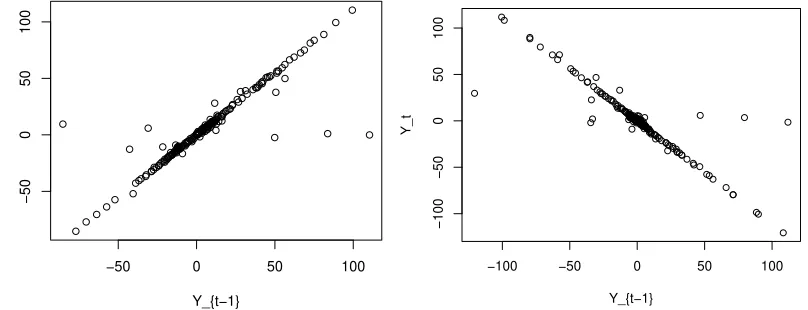
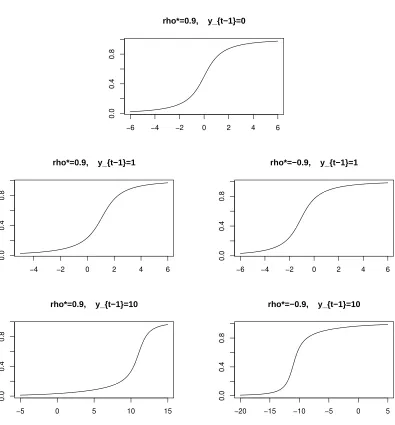
This can be illustrated by plotting Yt against Yt−1 for simulated paths of the noncausal

AR(1) process with Cauchy errors (see Figure 4). The theoretical result in Proposition

3.5 concerning the conditional mean is confirmed by the simulated data, the slopes being

almost equal to 1 and -1, respectively5

. However, we also observe plots almost on the line

Yt= 0. They correspond to the dates at which the large (multiple) bubbles collapse.

The difference between the rate of explosion of the bubble for a given trajectory and the

average rate of explosion of the process, equal to 1 under the martingale hypothesis, explains

why the standard UR tests often provide strange results. See e.g. Homm and Breitung

(2012) for a survey of UR tests for detecting bubbles, and Evans (1991), Charemza and

Deadman (1995) for pitfalls in testing for explosive bubbles.

Standard UR tests, based on a difference betweenρˆn and 1, will fail in detecting locally

explosive features in the noncausal AR Cauchy model, although the martingale property is

satisfied whenρ >0by Proposition 3.5. This is not surprising as the asymptotic properties

of standard UR tests are often derived under assumptions which are not satisfied by the

noncausal Cauchy AR(1) model, such as the non stationarity under the null hypothesis.

In our framework, a test for bubbles would need to detect successive transitory explosions

along the observed trajectory, and not an explosive behavior in average, or a breakpoint in

5_{In fact slightly larger than 1 and slightly smaller than}

−50 0 50 100

−50

0

50

100

Y_{t−1}

Y_t

−100 −50 0 50 100

−100

−50

0

50

100

Y_{t−1}

Y_t

Figure 4.Scatterplot ofYtagainstYt−1for the the Cauchy AR(1) simulation of Figure 3 withρ= 0.9

(left panel) andρ=₋0.9(right panel).

the explosive behavior in average, as in Busetti and Taylor (2004), Phillips et al. (2011) or

Phillips et al. (2015) approaches.

5.3. Diagnostic checking

After estimating the coefficientρ, it is important to verify the independence of the

resid-uals in (5.1). In this respect, diagnostic checks can be based on the first-order residual

autocorrelation. Let us define the backward residuals

ˆ ε∗

t =Yt−ρˆnYt+1, t= 1, . . . , n−1,

in the estimation of Model (5.1)-(5.2). Similarly, we define the forward residuals

ˆ

εt=Yt−ρˆnYt−1, t= 2, . . . , n.

To check the white noise property, we consider the (backward and forward) residuals

first-order autocorrelations defined by

R∗ n =

n_X−1

t=2

ˆ ε∗

tεˆ∗t−1/ n−1

X

t=1

(ˆε∗

t)2, Rn= n X

t=3

ˆ εtεˆt−1/

n X

t=2

ˆ ε2

t.

5.3.1. Asymptotic behaviour under correct specification

The asymptotic distributions of statisticsRn andR∗nunder model (5.1)-(5.2), that is under

Proposition 5.3. Let(Yt)be the strictly stationary solution of Model (5.1)-(5.2). Then

a2 n ˜ an

R∗n d

−→ρ2S1/S0− {1−ρ2}

∞ X

j=2

ρj−1Sj/S0, (5.7)

where the Sj are independent stable variables as described in Proposition 5.2. If α ≥ 1

and_|εt|is asymptotically equivalent to a Pareto, the statistic Rn has the same asymptotic

distribution asR∗

n. In particular, for the noncausal Cauchy AR process we have: n

lognR ∗ n

d

−→R and n

lognRn d

−→R, asn_{→ ∞},

withR=ρ(1 + 2ρ)Y X,whereX, Y are independent with Y ∼ C(0,1) andX ∼χ2_(1).

Similar results could be established for higher-order residual autocorrelations (see Lin and

McLeod (2008) for portmanteau tests in the case of causal AR processes with stable errors).

Thus, at least whenα≥1and the errors distribution is asymptotically equivalent to a

Pareto, the empirical autocorrelations of the residualsεˆ∗

t andεˆthave the same asymptotic behaviour. This is a consequence of the weak causal linear representation:

Yt=ρYt−1+ut, (5.8)

where theutare "empirically uncorrelated" variables, in the sense that, for any ℓ >0,

n X

t=ℓ+1

utut−ℓ/ n X

t=1

u2t →0, in probability asn→ ∞. (5.9)

In the standard case where errorsεt admit finite variance, (ut) is a weak white noise and

the same result is true. In our framework, the ut’s do not admit second-order moments.

A surprising difference with the classical case is the coexistence of the "empirically" weak

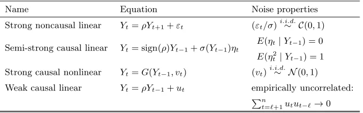
linear representation (5.8)-(5.9) and the semi-strong linear representation (3.6). Table 1

summarizes the different representations which can be defined for the noncausal Cauchy

AR(1) process.

5.3.2. Asymptotic behaviour of statistics under a (near) random walk

Let us now discuss the behavior of the statisticsRnandR∗nwhen the DGP is a strong AR(1)

with root at or near unity. More precisely, we consider a time series that is generated by

Yn,t=anYn,t−1+ξt, t≥1, an = exp(c/n), (5.10)

for some random initial valueY0whose distribution is independent ofnand of(ξt), wherec

Name Equation Noise properties Strong noncausal linear Yt=ρYt+1+εt (εt/σ)i.i.d.∼ C(0,1)

Semi-strong causal linear Yt=sign(ρ)Yt−1+σ(Yt−1)ηt

E(ηt|Yt−1) = 0

E(η2

t |Yt−1) = 1

Strong causal nonlinear Yt=G(Yt−1, vt) (vt)i.i.d.∼ N(0,1)

Weak causal linear Yt=ρYt−1+ut empirically uncorrelated: Pn

t=ℓ+1utut−ℓ→0

Table 1: Representations of the noncausal Cauchy AR(1) with|ρ|<1

for finiten, and it has explosive features forc >0. The errors may be dependent, but are

assumed to satisfy the following conditions:

A0: ξ= (ξt)is a strictly and second-order stationary process,E(ξt) = 0 andE(ξt2)>0.

A1: The strong mixing coefficients6

of the processξ are such that

∞ X

h=0

{αξ(h)}

ν

2+ν _{<∞ for someν >0, withE|ξ}

t|2+ν <∞.

Pham (1986) showed that A0-A1 hold for a large class of processes, the strong mixing coefficients converging to zero exponentially fast. As far as GARCH are concerned, results

on strict stationarity and strong mixing have been derived by numerous authors (see for

instance Chapter 3 in Francq and Zakoïan (2010) and the references therein). Note that

models (5.1)-(5.2) and (5.10) are non nested. Model (5.10), which was studied by Phillips

(1987) under slightly more general conditions thanA0-A1, might be erroneously estimated as a noncausal Cauchy AR in practice. The following result shows that the statisticsRnand

R∗

n computed from the process(Yn,t) have an asymptotic behavior which is very different from that obtained in Proposition 5.3.

Proposition 5.4. For the (near) random walk (5.10) underA0-A1, for anyc∈R:

n logn|R

∗

n| −→ ∞ and

n

logn|Rn| −→ ∞, in probability as n→ ∞.

Therefore, tests based onRn orRn∗, to be defined in Section 7, can distinguish a unit root

due to a stationary noncausal AR process from a unit root created by a (near) random walk

model.

6_{defined byα}

6. A Monte Carlo study

In this section, we study the behaviours of the estimatorρˆnand the statistics for diagnostic

checking introduced in Section 5.3. We also compareρˆn with the ML estimator ofρ.

6.1. Behaviour ofρˆnin finite samples

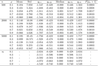
We simulatedN = 5,000paths of model (3.2) withα= 1andβ = 0, for different values of

ρ, ranging from 0.1 to 0.9, and different sample sizes (n=500, 2000, 5000). Table 2 shows

characteristics of the empirical distribution of _logn_n(ˆρn−ρ) over the N simulated paths.

Increasing the sample size does not entail much distorsion of the sample distributions,

indicating that the normalization by n

logn is appropriate for finite sample sizes. The median is always very small, and the first and third quartiles are rather close in modulus, at least

forρsufficiently far from 1, indicating thatρˆn is approximately symmetrically distributed

aroundρ. The probability ofρˆn exceeding 1 is extremely small, even forρ= 0.9, showing

that any standard unit-root test would reject the unit-root hypothesis. Comparison with the

asymptotic distribution in (5.6), see the casen=∞in Table 2, leads to mixed conclusions.

On the one hand, the center of the finite sample distributions (in the interquartile interval)

appears to be well approximated by the asymptotic distribution, at least forn sufficiently

large andρ not too close to 1. On the other hand, for ρ > 0, the absolute values of the

quantiles of the asymptotic distribution increase with ρ with a proportionality factor of

1 +ρ. This pattern does not appear in finite sample size for large values of ρ, and this is

particularly true for the extreme quantilesq0.1 andq0.9.

6.2. Statistics for diagnostic checking

Let us now study the statistics of Proposition 5.3. We only present, in Table 3, results

for the sample size n= 5000. The behaviour of the statisticsRn and R∗n is very similar,

whatever the values of n and ρ. The previous comments concerning the convergence to

the asymptotic distribution, that is the distribution of R, still apply. The two statistics

Rn and R∗n having the same asymptotic distribution, they cannot be used to distinguish

between a causal and a noncausal AR process. For this purpose, it can be useful to consider

n ρ Mean Std q0.1 q0.25 Median q0.75 q0.9 P[ˆρn>1] 500 0.1 0.104 7.050 -1.547 -0.428 -0.000 0.446 1.563 0.0003

0.3 0.101 5.324 -1.688 -0.482 0.000 0.488 1.659 0.0008 0.5 0.058 4.479 -1.811 -0.515 0.001 0.517 1.709 0.0017 0.7 -0.010 3.780 -1.791 -0.553 0.002 0.512 1.661 0.0033 0.9 -0.060 2.866 -1.544 -0.512 -0.004 0.450 1.301 0.0123 2000 0.1 0.140 16.08 -1.690 -0.423 0.003 0.429 1.657 0.0000 0.3 0.108 9.929 -1.838 -0.477 0.000 0.478 1.813 0.0002 0.5 0.079 8.187 -1.936 -0.524 -0.000 0.513 1.907 0.0006 0.7 0.021 6.650 -1.954 -0.549 -0.002 0.530 1.878 0.0010 0.9 -0.066 4.626 -1.707 -0.519 -0.003 0.495 1.578 0.0029 5000 0.1 0.195 35.45 -1.756 -0.422 0.000 0.432 1.717 0.0000 0.3 0.099 16.571 -1.928 -0.478 0.000 0.479 1.880 0.0001 0.5 -0.138 11.518 -2.054 -0.525 0.000 0.522 1.983 0.0002 0.7 0.021 9.255 -2.156 -0.551 0.000 0.544 2.032 0.0003 0.9 -0.053 6.947 -1.906 -0.541 0.000 0.511 1.808 0.0011

∞ 0.1 - - -2.634 -0.428 0.000 0.428 2.634

-0.3 - - -3.111 -0.506 0.000 0.506 3.111

-0.5 - - -3.592 -0.584 0.000 0.584 3.592

-0.7 - - -4.072 -0.662 0.000 0.662 4.072

-0.9 - - -4.549 -0.740 0.000 0.740 4.549

-Table 2: Characteristics of the empirical distribution of n

ρ q0.1 q0.25 Median q0.75 q0.9

R∗

n 0.1 -0.175 -0.045 0.000 0.047 0.195 0.3 -0.664 -0.170 0.000 0.173 0.695

0.5 -1.305 -0.337 0.000 0.345 1.339

0.7 -2.058 -0.535 0.001 0.545 2.068

0.9 -2.596 -0.724 0.001 0.749 2.731

Rn 0.1 -0.174 -0.045 0.000 0.047 0.194

0.3 -0.663 -0.170 0.000 0.173 0.692

0.5 -1.305 -0.337 0.000 0.341 1.327

0.7 -2.045 -0.538 0.000 0.536 2.027

0.9 -2.528 -0.719 0.000 0.719 2.599

R 0.1 -0.287 -0.047 0.000 0.047 0.287

0.3 -1.148 -0.187 0.000 0.187 1.148

0.5 -2.394 -0.390 0.000 0.390 2.394

0.7 -4.024 -0.654 0.000 0.654 4.024

0.9 -6.030 -0.981 0.000 0.981 6.030

Table 3: Characteristics of the empirical distributions of n

lognR ∗

ρ q0.1 q0.25 Median q0.75 q0.9

T∗

n 0.1 -0.595 -0.127 0.000 0.130 0.610 0.3 -0.606 -0.128 0.000 0.130 0.614

0.5 -0.610 -0.130 0.000 0.129 0.616

0.7 -0.635 -0.133 0.000 0.131 0.622

0.9 -0.651 -0.135 0.000 0.134 0.662

Tn 0.1 -51.33 -44.54 -0.220 44.19 51.11

0.3 -121.5 -105.3 0.139 104.8 121.0

0.5 -144.5 -125.2 -0.162 124.5 144.0

0.7 -82.62 -71.47 -0.272 71.07 82.16

0.9 -8.570 -7.384 -0.054 7.348 8.518

Table 4: Characteristics of the empirical distributions of _logn_nT∗

n and lognnTnover 5,000 simulated paths forn= 5,000.

residual. Let us consider the statistics:

Tn∗= n−1

X

t=2

ˆ

ε∗t(ˆε∗t−1)2/Dn∗, Tn= n X

t=3

ˆ

εt(ˆεt−1)2/Dn,

where D∗

n =

rPn−1 t=1(ˆε∗t)2

Pn−1 t=1(ˆε∗t)4

, and Dn = rPnt=1−1(ˆεt)2 Pnt=1−1(ˆεt)4

.

While(εt) is an i.i.d. sequence, the variables ut =Yt−ρYt−1 are only "empirically

un-correlated" [see (5.9)] and this should reflect in the behaviour of T∗

n andTn. The results presented in Table 4 confirm this intuition. The derivation of the asymptotic distributions

of such statistics is left for further research.

6.3. ML estimation of the non causal AR(1) Cauchy model

To gauge the efficiency loss due to the LS estimation of the non causal AR(1) Cauchy model,

we studied by Monte-Carlo experiments the properties of the ML estimator. Results are

displayed in Table 5. The efficiency loss of the LSE appears clearly by comparing Tables

5 and 2, but the MLE requires knowledge of the errors distribution which is a strong

n ρ Mean Std q0.1 q0.25 Median q0.75 q0.9

500 0.1 -0.020 4.190 -3.411 -1.029 -0.001 0.996 3.414 0.3 -0.049 3.633 -3.278 -1.010 -0.002 0.960 3.218 0.5 -0.063 3.023 -2.968 -0.960 -0.003 0.889 2.872 0.7 -0.073 2.334 -2.431 -0.824 -0.004 0.763 2.251 0.9 -0.069 1.370 -1.472 -0.509 -0.005 0.454 1.296 2000 0.1 -0.013 4.075 -3.477 -1.040 -0.000 1.011 3.409 0.3 -0.020 3.643 -3.280 -1.007 -0.003 0.984 3.221 0.5 -0.020 3.042 -2.935 -0.946 -0.001 0.917 2.877 0.7 -0.023 2.330 -2.378 -0.795 -0.000 0.775 2.319 0.9 -0.024 1.348 -1.428 -0.495 -0.001 0.481 1.368 5000 0.1 -0.012 4.323 -3.485 -1.051 -0.001 1.007 3.490 0.3 -0.018 3.721 -3.314 -1.019 -0.001 0.981 3.279 0.5 -0.017 3.074 -2.953 -0.961 -0.000 0.927 2.899 0.7 -0.012 2.358 -2.363 -0.807 -0.001 0.794 2.343 0.9 -0.007 1.372 -1.422 -0.492 0.000 0.489 1.404

Table 5: Characteristics of the empirical distribution ofn(ˆρM L,n−ρ)over 5,000 simulated paths of non causal AR(1) Cauchy models. The empiricalα-quantile is denotedqα.

7. An application

Many researchers found evidence of a speculative bubble in the series of the Nasdaq

com-posite price index (see Homm and Breitung (2012), Phillips et al. (2011), and the references

therein). Figure 5 plots the monthly time series of the Nasdaq real price7

from February

1973 to December 2012. To gauge the adequacy of the noncausal Cauchy AR(1) model,

we use the same data set as Phillips et al. (2011): the sample under study covers the

period from February 1973 to June 2005 and comprises 389 observations. We introduce the

statistics

Zn∗= n logn

R

∗ n ˆ

ρn(1 + 2 ˆρn)

, Zn= n logn

_{ρˆn(1 + 2 ˆ}Rn _ρn) .

Proposition 5.3 shows that the adequacy of the model is rejected at level α ∈ (0,1) if

Z∗

n > ζ1−α,where ζ1−α is the(1−α)quantile of the variable|XY|, using for instance the statisticsZ∗

n. The results displayed in Table 6 (left panel) show that the null hypothesis of a noncausal Cauchy AR(1) model cannot be rejected at any reasonable level for the tests

based onZn or Zn∗. The p-values are obtained from 1,000,000simulations of the variable

|Y_|X of Proposition 5.3. In view of Proposition 5.4, if the DGP was a unit-root or near unit-root model of the form (5.10) underA0-A1, the statistics Zn andZn∗ would converge

to infinity in probability. Thus, the probability that the p-value be arbitrarily close to 1

should converge to 1. The results clearly do not support this hypothesis. In other words,

the test procedures confirm what is seen on Figure 5. Indeed, the local explosive behaviour

is more visible than the slight global stochastic trend.

Finally, we estimated the Cauchy AR(1) model with Gaussian component in (4.7). To

compute the CF estimator, we used a discrete set up based on a grid(u1, λ1), . . . ,(um, λm)

for evaluating of the integral in (4.12). A preliminary estimator was obtained using a

uniform weighting functionW(_·). The estimator in (4.12) is thus obtained as

b

θn=arg min

θ_∈Θ

m X

i=1

|Ψen(ui, λiui)−Ψ(ui, λiui)|2.

We then considered the weight function

Wθ(u, λ) = [Var(cos{u(Zt+λZt+1)})]−1={0.5(1 + Ψ(2u,2λu))− {Ψ(u, λu)}2}−1.

where the CF function Ψ is evaluated at the parameterθ. The second step estimator is

thus obtained as

b

θ∗n=arg min

θ_∈Θ m X

i=1

|Ψen(ui, λiui)−Ψ(ui, λiui)|2Wθb_n(ui, λi).

The results of Table 6 (right panel) (obtained for the grid u _∈

{0.0005,0.001,0.01,0.1,0.5,1,2,3,5}andλ∈ {0.1,−0.2,0.5,−1,−0.5,1,2,−2,5}) confirm the existence of a non-causal Cauchy AR coefficient close to 1, while the Gaussian part

presents a relatively small AR coefficient. The causal part is thus clearly stationary.

ˆ

ρn Zn∗ Zn pval(Zn∗) pval(Zn)

0.998 0.980 1.030 0.341 0.333

ˆ

ρn rˆn ˆcn σˆn

0.978 0.263 1.377 1.048

Table 6: NASDAQ index : Testing adequacy of the Cauchy AR(1) model (left panel); Cauchy AR(1) model with a Gaussian component (right panel).

8. Concluding remarks

By considering a noncausal AR(1) process, with α-stable noncausal innovations, we have

derived special nonlinear features of its causal representation, such as locally explosive

0 100 200 300 400

200

400

600

800

1000

Figure 5.Real Nasdaq prices from February 1973 to December 2012.

features. The basic noncausal α-stable AR(1) process can be used as a cornerstone to

create local explosions in dynamic models, with different magnitudes and rates of explosion

by aggregation. We have seen that the noncausal Cauchy AR(1) process features a unit

root. This questions the interpretation of the unit root hypothesis. Indeed, a unit root

can represent a global explosive behaviour (stochastic trend) as well as a local explosion

(bubble). We discussed the interpretation of the standard tests introduced in the literature

to detect bubbles. These tests are often designed for detecting global explosions rather than

local ones. We also highlighted the possibility to predict the times at which bubbles collapse.

The analysis of our paper may help explain why mixed causal-noncausal linear AR models

with heavy-tailed errors provide good fit on a large number of macroeconomic and financial

time series. Indeed, these models are able to represent jumps, bubbles, and more generally

asymmetric peaks with different speeds of increase and decrease. Such nonlinear features

are often encountered in speculative markets, such as the market of physical commodities

or the market of electronic currencies as the bitcoin (see e.g. Gouriéroux, Hencic (2015)).

Appendix: Proofs and complementary results

A. Proofs

A.1. Proof of Proposition 3.1

Forα₆= 1, the characteristic function ofYt is

E[exp(ivYt)] = ∞ Y

h=0

E[exp{ivρhεt+h}]

= exp ∞ X

h=0

(−σα|v|α

|ρ|hαn₁

−iβ(signv) sign(ρ)htanπα

2 o

)

= exp

−σα|v|α

1 1_{− |}ρ_|α −

iβ(sign(v)) 1₋sign(ρ)_|ρ_|αtan

_πα 2 = exp − σ (1_{− |}ρ_|α₎1/α

α

|v_|α

1₋iβ(sign(v)) (1− |ρ| α₎

1−sign(ρ)|ρ|α tan _πα

2

.

This is the characteristic function of a stable distribution whose asymmetry parameter

depends on the sign ofρ. Forα= 1, we have

E[exp(ivYt)] = ∞ Y

h=0

E[exp_{ivρhεt+h}]

= exp (_∞

X

h=0

−σ|v||ρ|h

−ivβσ2

π ∞ X

h=0

ρhlog|vρh|

)

= exp

−σ_|v_|

1_{− |}ρ_| −ivβσ 2 π

log_|v_|

1₋ρ +

ρlog_|ρ_| (1₋ρ)2

.

A.2. Proof of Proposition 3.2

i) Let us first show that the causal Markov property holds (see also Cambanis and

Fakhre-Zakeri (1994), p. 217). Denote by f∗ the transition pdf in direct time and by f∗ the

transition pdf in reverse time. For any lagp, we have:

f_∗(Yt|Yt−1, . . . , Yt−p) =

f(Yt, Yt−1, . . . , Yt−p) f(Yt−1, . . . , Yt−p)

= f(Yt)f∗(Yt−1|Yt). . . f∗(Yt−p|Yt−p+1) f(Yt−1)f∗(Yt−2|Yt−1). . . f∗(Yt−p|Yt−p+1)

=f(Yt)f∗(Yt−1|Yt) f(Yt−1)

.

We deduce that the process(Yt)is also causal Markov, with causal transition:

f∗(Yt|Yt−1) =f(Yt)f

∗_(Yt −1|Yt) f(Yt−1)

ii) Now, the forward recursive equation at horizonh+ 1 is given by

Yt−1 = ρh+1Yt+h+εt−1+ρεt+. . .+ρhεt+h−1

= ρh+1_Y

t+h+εt−1,h, say.

The backward innovationεt−1,hat leadh+1follows a stable distribution with tail exponent

α. Letting fε,h denote the pdf of εt−1,h, the pdf of Yt−1 given Yt+h is thus the function

y_7→fε,h{y−ρh+1Yt+h}.By the Bayes formula, the pdf ofYt+h givenYt−1=y is thus the

function

g:x7→fε,h{y−ρh+1x}fY(x)/fY(y),

wherefY denotes the marginal pdf ofYt. If|β| 6= 1, the support of the stable pdf ofεt−1,h

andYt isR. It follows that whenx→ ±∞,

g(x)∼C(y)|x|−α−1

|y−ρh+1x|−α−1

∼C∗(y)|x|−2(α+1)_,

whereC(y)andC∗_{(y)are constants depending ony, which may change according to whether}

x→+∞or x→ −∞. Thus the integral of|x|p_{g(x)over any infinite interval excluding 0}

(resp. over any finite interval including 0) is finite iffp <2α+ 1 (resp. p >−1).

Now if |β| = 1, the support of the stable pdf of εt−1,h and Yt is either R+ or R−. It

follows that whenρh+1 _{>0, the support of the densityg is a compact; whenρ}h+1_{<0 it is}

bounded below or above. Thus we have established the proposition.

A.3. Proof of Proposition 3.3

Whenβ = 0, we have, by the arguments used to obtain Proposition 3.1,

Yt∼ S

α,0, σ

(1_{− |}ρ_|α₎1/α,0

, εt−1,h∼ S α,0, σ

1− |ρ|(h+1)α 1_{− |}ρ_|α

1/α ,0

! .

It follows that, for anyu_∈R,

E eiuYt−1

|Yt+h = eiuρ

h+1

Yt+h_{E e}iuεt−1,h _|Y t+h

= exp

iuρh+1Yt+h− |σu|α

1_{− |}ρ_|(h+1)α 1− |ρ|α

,

and thus for anyu, v_∈R,

E eiuYt−1+ivYt+h _{= EE e}iuYt−1

|Yt+h

eivYt+h

= exp

−|σu|α1− |ρ|(h+1)α

1_{− |}ρ_|α

Enei{v+uρh+1}Yt+h o

= exp

−|u_|α₍₁

− |ρ_|(h+1)α_{) +}

|v+uρh+1

|α σα

1− |ρ|α

Thus, foru >0and ρh+1_>0,

∂ ∂uE(e

iuYt−1+ivYt+h₎

v=0

= −E(eiuYt−1₎

|u|α−1₍₁

− |ρ|(h+1)α_{) +ρ}h+1

|uρh+1|α−1 ασα

1_{− |}ρ_|α

= −E(eiuYt−1₎

|u|α−1 ασα

1_{− |}ρ_|α, (A.2)

and

_∂

∂vE(e

iuYt−1+ivYt+h₎

v=0

= −E(eiuYt−1₎

|uρh+1|α−1 ασα

1− |ρ|α (A.3)

= ρ(h+1)(α−1)

∂ ∂uE(e

iuYt−1+ivYt+h₎

v=0

.

On the other hand, foru₆= 0,

∂ ∂uE(e

iuYt−1+ivYt+h₎

v=0

= iE(Yt−1eiuYt−1_),

∂ ∂vE(e

iuYt−1+ivYt+h₎

v=0

= iE(Yt+heiuYt−1).

Note that the latter expectations exist, by the Dirichlet’s test8

for improper integrals and

using the equivalent of the density of anα-stable variable in the neighborhood of infinity,

f(x)_∼ K

|x|α+1. Therefore, foru >0 andρ

h+1_>0,

EnYt+h−ρ(h+1)(α−1)Yt−1

eiuYt−1

o

= 0. (A.4)

It can be checked that foru < 0 and ρh+1 _{>0 both derivatives in (A.2) and (A.3) have}

opposite signs, thus (A.4) continues to hold. If nowρh+1_{<0, we obtain}

∂ ∂vE(e

iuYt−1+ivYt+h₎

v=0

= ₋(₋ρ)(h+1)(α−1)

∂ ∂uE(e

iuYt−1+ivYt+h₎

v=0

, ifα₆= 1

and

∂ ∂vE(e

iuYt−1+ivYt+h₎ v=0 = − ∂ ∂uE(e

iuYt−1+ivYt+h₎

v=0

ifα= 1.

Finally, we have

EnYt+h−sign(ρ)|ρ|(h+1)(α−1)Yt−1

eiuYt−1

o

= 0, for anyu_∈R. (A.5)

The conclusion follows from Bierens (Theorem 1, 1982).

8_{Let f and gdenote two real functions defined on[a,}

∞) and regulated on every interval[a, b]

withb > a(that is, admitting left-hand and right-hand limits at all pointsx > aand a right-hand limit at a). Iff is decreasing and limx→∞f(x) = 0, ifsupb|

Rb

ag(x)dx|<∞, then the integral R∞

A.4. Proof of Proposition 3.4

From the Proof of Proposition 3.2, the pdf ofYtgiven Yt−h=y is the function

g:x_7→fε,h−1{y−ρhx}fY(x)/fY(y),

where fY is the marginal pdf ofYt and fε,h−1 is the pdf ofPhi=0−1ρiεt−i. By Proposition

3.1,Yt∼ C

0, σ 1−|ρ|

, andfε,h−1 is the pdf of theC(0, σh). The conclusion follows.

A.5. Proof of Proposition 3.5

The proof of Proposition 3.5 uses the special form of the transition pdf and is given for

σ= 1andρ6= 0.

i) Let us first compute the conditional moment of1 + (1− |ρ|)2_Y2

t.We get:

Et−1[1 + (1− |ρ|)2Yt2] = Z +∞

−∞ 1 π

1

1 + (Yt−1−ρYt)2[1 + (1− |ρ|) 2_Y2

t−1]dYt

= 1

π[1 + (1− |ρ|)

2_Y2 t−1]

Z +∞

−∞

1

1 + (Yt−1−ρYt)2dYt

= 1

|ρ_|[1 + (1− |ρ|)

2_Y2 t−1].

We deduce the second equality in Proposition 3.5:

E(Yt2|Yt−1) = 1

|ρ_|Y

2 t−1+

1

|ρ_|(1_{− |}ρ_|). (A.6)

ii) By the same method, we can retrieve the conditional mean already obtained in

Propo-sition 3.3 using characteristic functions. Let us symmetrically compute:

Et−1[1 + (Yt−1−ρYt)2] = 1

π[1 + (1− |ρ|)

2_Y2 t−1]

Z −∞

−∞

1 1 + (1− |ρ|)2_Y2

t dYt

= 1

1_{− |}ρ_|[1 + (1− |ρ|)

2_Y2 t−1]

= 1

1− |ρ|+ (1− |ρ|)Y 2 t−1.

We deduce that:

2ρYt−1E(Yt|Yt−1) = 1 +Yt2−1+ρ2E(Yt2|Yt−1)−

1

1− |ρ| −(1− |ρ|)Y 2 t−1

= −₁ |ρ|

− |ρ_| +|ρ|Y

2

by applying expression (A.6). Therefore, we haveE(Yt|Yt−1) =signρYt−1,which provides

the first formula in Proposition 3.5.

A.6. Proof of Proposition 3.6

Since the transition pdf in reverse time being is given by:

f∗(Yt−1|Yt) = 1

√

2π

1 (Yt−1−ρYt)3/2

exp

−1

2(Yt−1−ρYt)

IYt−1−ρYt>0,

we deduce, by (A.1) and (3.7), the transition pdf in direct time is

f_∗(Yt|Yt−1) =

1

√

2π

Yt−1

Yt(Yt−1−ρYt) 3/2

exp

−1

2(1−√ρ)2

1 Yt−

1 Yt−1

×exp

−1

2(Yt−1−ρYt)

I0<ρYt<Yt−1.

The conclusion follows.

A.7. Proof of Proposition 4.1

We have

|Yt|=

Z X

i≥0

ρiερ,t+idπ(ρ) = X

i≥0

Xt,i

, Xt,i= Z

ρiερ,t+idπ(ρ).

To verify that_|Yt| is a.s. finite, it suffices to check that E|Yt|s < ∞. Note that, for any

integrable function H (with respect to π), the random variable R ερ,tH(ρ)dπ(ρ) follows a

Cauchy distribution with scale parameterEπ|H(ρ)|, provided the latter expectation is finite.

Therefore, the variableXt,i follows a Cauchy distribution with scale parameter Eπ(|ρ|i).

ThusE_|Xt,i|s ={Eπ(|ρ|i)}sms where, for s ∈ (0,1), ms is the s-th order moment of the

C(0,1).Using the elementary inequality (x+y)s ≤xs+ys forx, y ≥0 and s∈(0,1), we then have

E|Yt|s≤ X

i≥0

E|Xt,i|s= X

i≥0

{Eπ(|ρ|i)}sms<∞.

ThusYtis well defined and (4.4) holds. The Cauchy distribution of Ytfollows, noting that

Eπ n

1 1−|ρ|

o

exists under (4.3).

The strict stationarity of(ερ,t)t∈Z, for anyρ∈(−1,1), entails that the joint distribution

of any n-uple (_Yt1+h, . . . ,Ytn+h) does not depend of h. The strict stationarity of (Yt)

follows.

Let us now turn to ergodicity. Denote by (Ω,_B, P) the underlying probability space

and let Ω+ _{= R}Z+