Analyzing the Errors of Unsupervised Learning
Percy Liang Dan Klein
Computer Science Division, EECS Department University of California at Berkeley
Berkeley, CA 94720 {pliang,klein}@cs.berkeley.edu
Abstract
We identify four types of errors that unsu-pervised induction systems make and study each one in turn. Our contributions include (1) using ameta-modelto analyze the incor-rect biases of a model in a systematic way, (2) providing an efficient and robust method of measuring distance between two parameter settings of a model, and (3) showing that lo-cal optima issues which typilo-cally plague EM can be somewhat alleviated by increasing the number of training examples. We conduct our analyses on three models: the HMM, the PCFG, and a simple dependency model.
1 Introduction
The unsupervised induction of linguistic structure from raw text is an important problem both for un-derstanding language acquisition and for building language processing systems such as parsers from limited resources. Early work on inducing gram-mars via EM encountered two serious obstacles: the inappropriateness of the likelihood objective and the tendency of EM to get stuck in local optima. With-out additional constraints on bracketing (Pereira and Shabes, 1992) or on allowable rewrite rules (Carroll and Charniak, 1992), unsupervised grammar learn-ing was ineffective.
Since then, there has been a large body of work addressing the flaws of the EM-based approach. Syntactic models empirically more learnable than PCFGs have been developed (Clark, 2001; Klein and Manning, 2004). Smith and Eisner (2005) pro-posed a new objective function; Smith and Eis-ner (2006) introduced a new training procedure. Bayesian approaches can also improve performance (Goldwater and Griffiths, 2007; Johnson, 2007; Kurihara and Sato, 2006).
Though these methods have improved induction accuracy, at the core they all still involve optimizing non-convex objective functions related to the like-lihood of some model, and thus are not completely immune to the difficulties associated with early ap-proaches. It is therefore important to better under-stand the behavior of unsupervised induction sys-tems in general.
In this paper, we take a step back and present a more statistical view of unsupervised learning in the context of grammar induction. We identify four
types of error that a system can make:
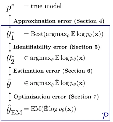
approxima-tion,identifiability,estimation, andoptimization er-rors (see Figure 1). We try to isolate each one in turn and study its properties.
Approximation error is caused by a mis-match between the likelihood objective optimized by EM and the true relationship between sentences and their syntactic structures. Our key idea for understand-ing this mis-match is to “cheat” and initialize EM with the true relationship and then study the ways in which EM repurposes our desired syntactic
struc-tures to increase likelihood. We present a
meta-modelof the changes that EM makes and show how this tool can shed some light on the undesired biases of the HMM, the PCFG, and the dependency model with valence (Klein and Manning, 2004).
Identifiability error can be incurred when two dis-tinct parameter settings yield the same probabil-ity distribution over sentences. One type of non-identifiability present in HMMs and PCFGs is label symmetry, which even makes computing a mean-ingful distance between parameters NP-hard. We present a method to obtain lower and upper bounds on such a distance.
Estimation error arises from having too few train-ing examples, and optimization error stems from
EM getting stuck in local optima. While it is to be expected that estimation error should decrease as the amount of data increases, we show that optimization error can also decrease. We present striking experi-ments showing that if our data actually comes from the model family we are learning with, we can some-times recover the true parameters by simply run-ning EM without clever initialization. This result runs counter to the conventional attitude that EM is doomed to local optima; it suggests that increasing the amount of data might be an effective way to par-tially combat local optima.
2 Unsupervised models
Letxdenote an input sentence andydenote the
un-observed desired output (e.g., a parse tree). We con-sider a model familyP ={pθ(x,y) : θ ∈Θ}. For
example, ifP is the set of all PCFGs, then the
pa-rametersθwould specify all the rule probabilities of
a particular grammar. We sometimes useθ andpθ
interchangeably to simplify notation. In this paper, we analyze the following three model families:
In theHMM, the inputxis a sequence of words
and the output y is the corresponding sequence of
part-of-speech tags.
In the PCFG, the inputx is a sequence of POS
tags and the outputyis a binary parse tree with yield
x. We representyas a multiset of binary rewrites of the form(y→ y1y2), whereyis a nonterminal and
y1, y2 can be either nonterminals or terminals.
In the dependency model with valence (DMV)
(Klein and Manning, 2004), the input x =
(x1, . . . , xm)is a sequence of POS tags and the
out-putyspecifies the directed links of a projective de-pendency tree. The generative model is as follows:
for each head xi, we generate an independent
se-quence of arguments to the left and to the right from a direction-dependent distribution over tags. At each point, we stop with a probability parametrized by the direction and whether any arguments have already been generated in that direction. See Klein and Man-ning (2004) for a formal description.
In all our experiments, we used the Wall Street Journal (WSJ) portion of the Penn Treebank. We bi-narized the PCFG trees and created gold dependency trees according to the Collins head rules. We trained 45-state HMMs on all 49208 sentences, 11-state
PCFGs on WSJ-10 (7424 sentences) and DMVs on WSJ-20 (25523 sentences) (Klein and Manning, 2004). We ran EM for 100 iterations with the pa-rameters initialized uniformly (always plus a small amount of random noise). We evaluated the HMM and PCFG by mapping model states to Treebank tags to maximize accuracy.
3 Decomposition of errors
Now we will describe the four types of errors (Fig-ure 1) more formally. Letp∗(x,y)denote the distri-bution which governs the true relationship between
the inputx and output y. In general, p∗ does not
live in our model familyP. We are presented with
a set ofnunlabeled examplesx(1), . . . ,x(n)drawn i.i.d. from the true p∗. In unsupervised induction, our goal is to approximatep∗by some modelpθ ∈ P
in terms of strong generative capacity. A standard approach is to use the EM algorithm to optimize the empirical likelihoodEˆlogpθ(x).1However, EM
only finds a local maximum, which we denoteθˆEM,
so there is adiscrepancybetween what we get (pθˆEM)
and what we want (p∗).
We will define this discrepancy later, but for now, it suffices to remark that the discrepancy depends
on the distribution overywhereas learning depends
only on the distribution overx. This is an important property that distinguishes unsupervised induction from more standard supervised learning or density estimation scenarios.
Now let us walk through the four types of
er-ror bottom up. First, θˆEM, the local maximum
found by EM, is in general different from θˆ ∈
argmaxθEˆlogpθ(x), any global maximum, which
we could find given unlimited computational
re-sources. Optimization error refers to the
discrep-ancy betweenθˆandθˆEM.
Second, our training data is only a noisy
sam-ple from the true p∗. If we had infinite data, we
would choose an optimal parameter setting under the model, θ2∗ ∈ argmaxθElogpθ(x), where now the
expectationEis taken with respect to the truep∗
in-stead of the training data. The discrepancy between
θ2∗andθˆis theestimation error.
Note that θ2∗ might not be unique. Letθ∗1 denote
1Here, the expectationˆ
Ef(x) def= 1n
Pn i=1f(x
(i))denotes
p
∗ = true modelApproximation error (Section 4)
θ
1∗ = Best(argmaxθElogpθ(x))Identifiability error (Section 5)
θ
2∗ ∈argmaxθElogpθ(x)Estimation error (Section 6)
ˆ
θ
∈argmaxθEˆlogpθ(x) Optimization error (Section 7)ˆ
[image:3.612.96.278.55.250.2]θ
EM= EM(ˆElogpθ(x))P
Figure 1: The discrepancy between what we get (θˆEM)
and what we want (p∗) can be decomposed into four types of errors. The box represents our model familyP, which is the set of possible parametrized distributions we can represent. Best(S)returns theθ∈Swhich has the small-est discrepancy withp∗.
the maximizer of Elogpθ(x) that has the smallest
discrepancy withp∗. Sinceθ∗1andθ∗2 have the same value under the objective function, we would not be able to chooseθ∗1 overθ2∗, even with infinite data or unlimited computation. Identifiability error refers to the discrepancy betweenθ1∗andθ2∗.
Finally, the model familyP has fundamental
lim-itations. Approximation errorrefers to the
discrep-ancy betweenp∗ andpθ∗
1. Note that θ
∗
1 is not
nec-essarily the best inP. If we had labeled data, we
could find a parameter setting inP which is closer
to p∗ by optimizing joint likelihood Elogpθ(x,y)
(generative training) or even conditional likelihood
Elogpθ(y|x)(discriminative training).
In the remaining sections, we try to study each of the four errors in isolation. In practice, since it is difficult to work with some of the parameter settings that participate in the error decomposition, we use computationally feasible surrogates so that the error under study remains the dominant effect.
4 Approximation error
We start by analyzing approximation error, the
dis-crepancy between p∗ andpθ∗1 (the model found by
optimizing likelihood), a point which has been
dis-20 40 60 80 100 iteration -18.4
-18.0 -17.6 -17.2 -16.7
log-lik
eliho
o
d
20 40 60 80 100 iteration 0.2
0.4 0.6 0.8 1.0
Lab
eled
[image:3.612.311.546.60.152.2]F1
Figure 2: For the PCFG, when we initialize EM with the supervised estimateθˆgen, the likelihood increases but the
accuracy decreases.
cussed by many authors (Merialdo, 1994; Smith and
Eisner, 2005; Haghighi and Klein, 2006).2
To confront the question of specifically how the likelihood diverges from prediction accuracy,
we perform the following experiment: we
ini-tialize EM with the supervised estimate3 θˆgen =
argmaxθEˆlogpθ(x,y), which acts as a surrogate
forp∗. As we run EM, the likelihood increases but
the accuracy decreases (Figure 2 shows this trend for the PCFG; the HMM and DMV models behave similarly). We believe that the initial iterations of EM contain valuable information about the incor-rect biases of these models. However, EM is chang-ing hundreds of thousands of parameters at once in a non-trivial way, so we need a way of characterizing the important changes.
One broad observation we can make is that the first iteration of EM reinforces the systematic mis-takes of the supervised initializer. In the first E-step, the posterior counts that are computed summarize the predictions of the supervised system. If these match the empirical counts, then the M-step does not change the parameters. But if the supervised system predicts too many JJs, for example, then the M-step will update the parameters to reinforce this bias.
4.1 A meta-model for analyzing EM
We would like to go further and characterize the specific changes EM makes. An initial approach is to find the parameters that changed the most dur-ing the first iteration (weighted by the
correspond-2Here, we think of discrepancy betweenpandp0
as the error incurred when usingp0 for prediction on examples generated fromp; in symbols,E(x,y)∼ploss(y,argmaxy0p0(y0|x)).
3For all our models, the supervised estimate is solved in
ing expected counts computed in the E-step). For the HMM, the three most changed parameters are
the transitions 2:DT→8:JJ, START→0:NNP, and
8:JJ→3:NN.4 If we delve deeper, we can see that
2:DT→3:NN (the parameter with the 10th largest
change) fell and 2:DT→8:JJ rose. After checking
with a few examples, we can then deduce that some nouns were retagged as adjectives. Unfortunately, this type of ad-hoc reasoning requires considerable manual effort and is rather subjective.
Instead, we propose using a general meta-model
to analyze the changes EM makes in an automatic and objective way. Instead of treating parameters as the primary object of study, we look at predictions made by the model and study how they change over time. While a model is a distribution over sentences, a meta-model is a distribution over how the predic-tions of the model change.
Let R(y) denote the set of parts of a
predic-tion ythat we are interested in tracking. Each part
(c, l)∈R(y)consists of aconfigurationcand a lo-cationl. For a PCFG, we define a configuration to be a rewrite rule (e.g.,c=PP→IN NP), and a loca-tionl = [i, k, j]to be a span[i, j]split atk, where the rewritecis applied.
In this work, each configuration is associated with a parameter of the model, but in general, a configu-ration could be a larger unit such as a subtree, allow-ing one to track more complex changes. The size of a configuration governs how much the meta-model generalizes from individual examples.
Lety(i,t) denote the model prediction on thei-th
training example after t iterations of EM. To
sim-plify notation, we writeRt = R(y(i,t)). The
meta-model explains howRtbecameRt+1.5
In general, we expect a part in Rt+1 to be
ex-plained by a part in Rt that has a similar location
and furthermore, we expect the locations of the two parts to be related in some consistent way. The meta-model uses two notions to formalize this idea: a dis-tance d(l, l0) and a relationr(l, l0). For the PCFG,
d(l, l0) is the number of positions amongi,j,k that
are the same as the corresponding ones in l0, and
r((i, k, j),(i0, k0, j0)) = (sign(i − i0),sign(j −
4Here 2:DT means state 2 of the HMM, which was greedily
mapped to DT.
5If the same part appears in bothR
tandRt+1, we remove
it from both sets.
j0),sign(k−k0))is one of 33 values. We define a
migrationas a triple(c, c0, r(l, l0)); this is the unit of change we want to extract from the meta-model.
Our meta-model provides the following
genera-tive story of howRtbecomes Rt+1: each new part
(c0, l0) ∈ Rt+1chooses an old part(c, l) ∈Rtwith
some probability that depends on (1) the distance be-tween the locationslandl0and (2) the likelihood of the particular migration. Formally:
pmeta(Rt+1 |Rt) =
Y
(c0,l0)∈R t+1
X
(c,l)∈Rt
Zl−01e−αd(l,l 0)
p(c0 |c, r(l, l0)),
whereZl = P(c,l)∈Rte
−αd(l,l0) is a normalization
constant, andα is a hyperparameter controlling the
possibility of distant migrations (set to 3 in our ex-periments).
We learn the parameters of the meta-model with an EM algorithm similar to the one for IBM model 1. Fortunately, the likelihood objective is convex, so we need not worry about local optima.
4.2 Results of the meta-model
We used our meta-model to analyze the approxima-tion errors of the HMM, DMV, and PCFG. For these models, we initialized EM with the supervised es-timate θˆgen and collected the model predictions as
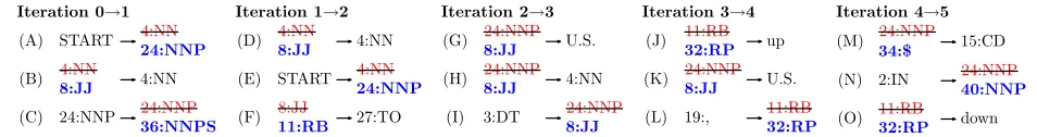
EM ran. We then trained the meta-model on the pre-dictions between successive iterations. The meta-model gives us an expected count for each migra-tion. Figure 3 lists the migrations with the highest expected counts.
From these migrations, we can see that EM tries
to explainx better by making the correspondingy
more regular. In fact, many of the HMM migra-tions on the first iteration attempt to resolve incon-sistencies in gold tags. For example, noun adjuncts (e.g.,stock-index), tagged as both nouns and adjec-tives in the Treebank, tend to become consolidated under adjectives, as captured by migration (B). EM also re-purposes under-utilized states to better cap-ture distributional similarities. For example, state 24 has migrated to state 40 (N), both of which are now dominated by proper nouns. State 40 initially con-tained only #, but was quickly overrun with
distribu-tionally similar proper nouns such asOct.and
Iteration 0→1
(A) START 4:NN 24:NNP
(B) 4:NN
8:JJ 4:NN
(C) 24:NNP 24:NNP 36:NNPS
Iteration 1→2
(D) 4:NN
8:JJ 4:NN
(E) START 4:NN 24:NNP
(F) 8:JJ
11:RB 27:TO
Iteration 2→3
(G) 24:NNP 8:JJ U.S.
(H) 24:NNP 8:JJ 4:NN
(I) 3:DT 24:NNP 8:JJ
Iteration 3→4
(J) 11:RB 32:RP up
(K) 24:NNP 8:JJ U.S.
(L) 19:, 11:RB 32:RP
Iteration 4→5
(M) 24:NNP 34:$ 15:CD
(N) 2:IN 24:NNP 40:NNP
(O) 11:RB
32:RP down
(a) Top HMM migrations. Example: migration (D) means aNN→NNtransition is replaced byJJ→NN.
Iteration 0→1 Iteration 1→2 Iteration 2→3 Iteration 3→4 Iteration 4→5
(A) DT NN NN (D) NNP NNP NNP (G) DT JJ NNS (J) DT JJ NN (M) POS JJ NN
(B) JJ NN NN (E) NNP NNP NNP (H) MD RB VB (K) DT NNP NN (N) NNS RB VBP
(C) NNP NNP (F) DT NNP NNP (I) VBP RB VB (L) PRP$ JJ NN (O) NNS RB VBD
(b) Top DMV migrations. Example: migration (A) means a DT attaches to the closer NN.
Iteration 0→1 Iteration 1→2 Iteration 2→3 Iteration 3→4 Iteration 4→5
(A) RB 1:VP 4:S RB 1:VP 1:VP (D) NNP 0:NP 0:NP NNP NNP 0:NP (G) DT 0:NP 0:NP DT NN 0:NP (J) TO VB 1:VP TO VB 2:PP (M) CD NN 0:NP CD NN 3:ADJP (B) 0:NP 2:PP 0:NP 1:VP 2:PP 1:VP (E) VBN 2:PP 1:VP 1:VP 2:PP 1:VP (H) 0:NP 1:VP 4:S 0:NP 1:VP 4:S (K) MD 1:VP 1:VP MD VB 1:VP (N) VBD 0:NP 1:VP VBD3:ADJP 1:VP (C) VBZ 0:NP 1:VP VBZ 0:NP 1:VP (F) 0:NP 1:VP 4:S 0:NP 1:VP 4:S (I) TO VB 1:VP TO VB 2:PP (L) NNP NNP 0:NP NNP NNP 6:NP (O) 0:NP NN 0:NP 0:NP NN 0:NP
[image:5.612.66.543.58.121.2](c) Top PCFG migrations. Example: migration (D) means aNP→NNP NPrewrite is replaced byNP→NNP NNP, where the new NNP right child spans less than the old NP right child.
Figure 3: We show the prominent migrations that occur during the first 5 iterations of EM for the HMM, DMV, and PCFG, as recovered by our meta-model. We sort the migrations across each iteration by their expected counts under the meta-model and show the top 3. Iteration 0 corresponds to the correct outputs. Blue indicates the new iteration, red indicates the old.
DMV migrations also try to regularize model pre-dictions, but in a different way—in terms of the number of arguments. Because the stop probability is different for adjacent and non-adjacent arguments, it is statistically much cheaper to generate one argu-ment rather than two or more. For example, if we train a DMV on only DT JJ NN, it can fit the data perfectly by using a chain of single arguments, but perfect fit is not possible if NN generates both DT and JJ (which is the desired structure); this explains migration (J). Indeed, we observed that the variance of the number of arguments decreases with more EM iterations (for NN, from 1.38 to 0.41).
In general, low-entropy conditional distributions are preferred. Migration (H) explains how adverbs now consistently attach to verbs rather than modals. After a few iterations, the modal has committed itself to generating exactly one verb to the right,
which is statistically advantageous because there must be a verb after a modal, while the adverb is op-tional. This leaves the verb to generate the adverb.
The PCFG migrations regularize categories in a manner similar to the HMM, but with the added complexity of changing bracketing structures. For example, sentential adverbs are re-analyzed as VP adverbs (A). Sometimes, multiple migrations
ex-plain the same phenomenon.6 For example,
migra-tions (B) and (C) indicate that PPs that previously attached to NPs are now raised to the verbal level. Tree rotation is another common phenomenon, lead-ing to many left-branchlead-ing structures (D,G,H). The migrations that happen during one iteration can also trigger additional migrations in the next. For exam-ple, the raising of the PP (B,C) inspires more of the
6We could consolidate these migrations by using larger
same raising (E). As another example, migration (I) regularizes TO VB infinitival clauses into PPs, and this momentum carries over to the next iteration with even greater force (J).
In summary, the meta-model facilitates our anal-yses by automatically identifying the broad trends. We believe that the central idea of modeling the er-rors of a system is a powerful one which can be used to analyze a wide range of models, both supervised and unsupervised.
5 Identifiability error
While approximation error is incurred when likeli-hood diverges from accuracy, identifiability error is concerned with the case where likelihood is indiffer-ent to accuracy.
We say a set of parameters S is identifiable (in
terms ofx) if pθ(x) 6= pθ0(x) for every θ, θ0 ∈ S where θ 6= θ0.7 In general, identifiability error is incurred when the set of maximizers ofElogpθ(x)
is non-identifiable.8
Label symmetry is perhaps the most familiar ex-ample of non-identifiability and is intrinsic to mod-els with hidden labmod-els (HMM and PCFG, but not DMV). We can permute the hidden labels without changing the objective function or even the nature of the solution, so there is no reason to prefer one permutation over another. While seemingly benign, this symmetry actually presents a serious challenge in measuring discrepancy (Section 5.1).
Grenager et al. (2005) augments an HMM to al-low emission from a generic stopword distribution at
any position with probabilityq. Their model would
definitely not be identifiable ifqwere a free param-eter, since we can setqto 0 and just mix in the stop-word distribution with each of the other emission distributions to obtain a different parameter setting yielding the same overall distribution. This is a case where our notion of desired structure is absent in the likelihood, and a prior over parameters could help break ties.
7
For our three model families,θis identifiable in terms of (x,y), but not in terms ofxalone.
8
We emphasize that non-identifiability is in terms ofx, so two parameter settings could still induce the same marginal dis-tribution onx(weak generative capacity) while having different joint distributions on(x,y)(strong generative capacity). Recall that discrepancy depends on the latter.
The above non-identifiabilities apply to all param-eter settings, but another type of non-identifiability concerns only the maximizers ofElogpθ(x).
Sup-pose the true data comes from aK-state HMM. If
we attempt to fit an HMM with K + 1 states, we
can split any one of theK states and maintain the
same distribution onx. Or, if we learn a PCFG on
the same HMM data, then we can choose either the left- or right-branching chain structures, which both mimic the true HMM equally well.
5.1 Permutation-invariant distance
KL-divergence is a natural measure of discrepancy between two distributions, but it is somewhat non-trivial to compute—for our three recursive models, it requires solving fixed point equations, and becomes completely intractable in face of label symmetry. Thus we propose a more manageable alternative:
dµ(θ||θ0)
def =
P
jµj|θj−θ 0 j|
P
jµj
, (1)
where we weight the difference between the j-th
component of the parameter vectors by µj, the j
-th expected sufficient statistic wi-th respect to pθ
(the expected counts computed in the E-step).9
Un-like KL, our distancedµ is only defined on
distri-butions in the model family and is not invariant to
reparametrization. Like KL,dµis asymmetric, with
the first argument holding the status of being the “true” parameter setting. In our case, the parameters are conditional probabilities, so0≤dµ(θ||θ0)≤1,
so we can interpretdµas an expected difference
be-tween these probabilities.
Unfortunately, label symmetry can wreak havoc
on our distance measure dµ. Suppose we want to
measure the distance between θ and θ0. If θ0 is
simplyθ with the labels permuted, then dµ(θ||θ0)
would be substantial even though the distance ought to be zero. We define a revised distance to correct for this by taking the minimum distance over all la-bel permutations:
Dµ(θ||θ0) = min
π dµ(θ||π(θ
0)), (2)
9
where π(θ0) denotes the parameter setting
result-ing from permutresult-ing the labels accordresult-ing toπ. (The
DMV has no label symmetries, so justdµworks.)
For mixture models, we can compute Dµ(θ||θ0)
efficiently as follows. Note that each term in the
summation of (1) is associated with one of the K
labels. We can form aK×KmatrixM, where each
entryMij is the distance between the parameters
in-volving labeliofθand labeljofθ0.Dµ(θ||θ0)can
then be computed by finding a maximum weighted
bipartite matching onM using theO(K3)
Hungar-ian algorithm (Kuhn, 1955).
For models such as the HMM and PCFG, com-putingDµis NP-hard, since the summation indµ(1)
contains both first-order terms which depend on one label (e.g., emission parameters) and higher-order terms which depend on more than one label (e.g., transitions or rewrites). We cannot capture these
problematic higher-order dependencies inM.
However, we can bound Dµ(θ||θ0) as follows.
We create M using only first-order terms and find
the best matching (permutation) to obtain a lower
boundDµand an associated permutationπ0
achiev-ing it. SinceDµ(θ||θ0)takes the minimum over all
permutations, dµ(θ||π(θ0)) is an upper bound for
anyπ, in particular forπ=π0. We then use a local
search procedure that changes π to further tighten
the upper bound. LetDµdenote the final value.
6 Estimation error
Thus far, we have considered approximation and identifiability errors, which have to do with flaws of the model. The remaining errors have to do with how well we can fit the model. To focus on these errors, we consider the case where the true model is in our family (p∗ ∈ P). To keep the setting as real-istic as possible, we do supervised learning on real labeled data to obtain θ∗ = argmaxθEˆlogp(x,y).
We then throw away our real data and letp∗ =pθ∗. Now we start anew: sample new artificial data from
θ∗, learn a model using this artificial data, and see how close we get to recoveringθ∗.
In order to compute estimation error, we need to compareθ∗withθˆ, the global maximizer of the like-lihood on our generated data. However, we cannot computeθˆexactly. Let us therefore first consider the simpler supervised scenario. Here,θgenˆ has a closed
form solution, so there is no optimization error. Us-ing our distanceDµ(defined in Section 5.1) to
quan-tify estimation error, we see that, for the HMM,θˆgen
quickly approachesθ∗as we increase the amount of
data (Table 1).
# examples 500 5K 50K 500K
Dµ(θ∗||θˆgen) 0.003 6.3e-4 2.7e-4 8.5e-5
Dµ(θ∗||θˆgen) 0.005 0.001 5.2e-4 1.7e-4
Dµ(θ∗||θˆgen-EM) 0.022 0.018 0.008 0.002 Dµ(θ∗||θˆgen-EM) 0.049 0.039 0.016 0.004
Table 1: Lower and upper bounds on the distance from the trueθ∗ for the HMM as we increase the number of examples.
In the unsupervised case, we use the following procedure to obtain a surrogate forθˆ: initialize EM
with the supervised estimate θˆgen and run EM for
100 iterations. Letθgen-EMˆ denote the final param-eters, which should be representative ofθˆ. Table 1 shows that the estimation error ofθˆgen-EMis an order
of magnitude higher than that ofθˆgen, which is to
ex-pected sinceθˆgen-EMdoes not have access to labeled
data. However, this error can also be driven down given a moderate number of examples.
7 Optimization error
Finally, we study optimization error, which is the
discrepancy between the global maximizer θˆ and
ˆ
θEM, the result of running EM starting from a
uni-form initialization (plus some small noise). As be-fore, we cannot computeθˆ, so we use θˆgen-EM as a
surrogate. Also, instead of comparingθˆgen-EMandθˆ
with each other, we compare each of their discrep-ancies with respect toθ∗.
Let us first consider optimization error in terms
of prediction error. The first observation is that
there is a gap between the prediction accuracies
of θgen-EMˆ and θEMˆ , but this gap shrinks
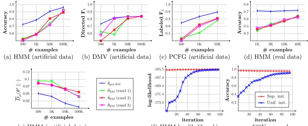
consider-ably as we increase the number of examples. Fig-ures 4(a,b,c) support this for all three model fami-lies: for the HMM, bothθgen-EMˆ andθEMˆ eventually achieve around 90% accuracy; for the DMV, 85%. For the PCFG,θˆEMstill lagsθˆgen-EMby 10%, but we
500 5K 50K 500K
# examples
0.6 0.7 0.8 0.9 1.0
Accuracy
500 5K 50K 500K
# examples
0.6 0.7 0.8 0.9 1.0
Directed
F1
500 5K 50K
# examples
0.5 0.6 0.8 0.9 1.0
Lab
eled
F1
1K 3K 10K 40K
# examples
0.3 0.4 0.6 0.7 0.8
Accuracy
(a) HMM (artificial data) (b) DMV (artificial data) (c) PCFG (artificial data) (d) HMM (real data)
500 5K 50K 500K
# examples
0.02 0.05 0.07 0.1 0.12
D
µ
(
θ
∗||
·
) ˆ
θgen-EM
ˆ
θEM(rand 1)
ˆ
θEM(rand 2)
ˆ
θEM(rand 3)
20 40 60 80 100
iteration
-173.3 -171.4 -169.4 -167.4 -165.5
log-lik
eliho
o
d
20 40 60 80 100
iteration
0.2 0.4 0.6 0.8 1.0
Accuracy Sup. init.Unif. init.
[image:8.612.67.558.60.261.2](e) HMM (artificial data) (f) HMM log-likelihood/accuracy on 500K examples
Figure 4: Compares the performance ofθˆEM(EM with a uniform initialization) againstθˆgen-EM(EM initialized with the
supervised estimate) on (a–c) various models, (d) real data. (e) measures distance instead of accuracy and (f) shows a sample EM run.
between θgen-EMˆ and θEMˆ also diminishes for the
HMM. To reaffirm the trends, we also measure
dis-tanceDµ. Figure 4(e) shows that the distance from
ˆ
θEMto the true parametersθ∗ decreases, but the gap
between θˆgen-EM and θˆEM does not close as
deci-sively as it did for prediction error.
It is quite surprising that by simply running EM with a neutral initialization, we can accurately learn a complex model with thousands of parameters. Fig-ures 4(f,g) show how both likelihood and accuracy, which both start quite low, improve substantially over time for the HMM on artificial data.
Carroll and Charniak (1992) report that EM fared poorly with local optima. We do not claim that there are no local optima, but only that the likelihood sur-face that EM is optimizing can become smoother with more examples. With more examples, there is less noise in the aggregate statistics, so it might be easier for EM to pick out the salient patterns.
Srebro et al. (2006) made a similar observation in the context of learning Gaussian mixtures. They characterized three regimes: one where EM was suc-cessful in recovering the true clusters (given lots of data), another where EM failed but the global opti-mum was successful, and the last where both failed (without much data).
There is also a rich body of theoretical work on
learning latent-variable models. Specialized algo-rithms can provably learn certain constrained dis-crete hidden-variable models, some in terms of weak generative capacity (Ron et al., 1998; Clark and Thollard, 2005; Adriaans, 1999), others in term of strong generative capacity (Dasgupta, 1999; Feld-man et al., 2005). But with the exception of Das-gupta and Schulman (2007), there is little theoretical understanding of EM, let alone on complex model families such as the HMM, PCFG, and DMV.
8 Conclusion
References
P. W. Adriaans. 1999. Learning shallow context-free lan-guages under simple distributions. Technical report, Stanford University.
G. Carroll and E. Charniak. 1992. Two experiments on learning probabilistic dependency grammars from cor-pora. InWorkshop Notes for Statistically-Based NLP Techniques, pages 1–13.
A. Clark and F. Thollard. 2005. PAC-learnability of probabilistic deterministic finite state automata.
JMLR, 5:473–497.
A. Clark. 2001. Unsupervised induction of stochastic context free grammars with distributional clustering. InCoNLL.
S. Dasgupta and L. Schulman. 2007. A probabilistic analysis of EM for mixtures of separated, spherical Gaussians. JMLR, 8.
S. Dasgupta. 1999. Learning mixtures of Gaussians. In
FOCS.
J. Feldman, R. O’Donnell, and R. A. Servedio. 2005. Learning mixtures of product distributions over dis-crete domains. InFOCS, pages 501–510.
S. Goldwater and T. Griffiths. 2007. A fully Bayesian approach to unsupervised part-of-speech tagging. In
ACL.
T. Grenager, D. Klein, and C. D. Manning. 2005. Un-supervised learning of field segmentation models for information extraction. InACL.
A. Haghighi and D. Klein. 2006. Prototype-based gram-mar induction. InACL.
M. Johnson. 2007. Why doesn’t EM find good HMM POS-taggers? InEMNLP/CoNLL.
D. Klein and C. D. Manning. 2004. Corpus-based induc-tion of syntactic structure: Models of dependency and constituency. InACL.
H. W. Kuhn. 1955. The Hungarian method for the as-signment problem. Naval Research Logistic Quar-terly, 2:83–97.
K. Kurihara and T. Sato. 2006. Variational Bayesian grammar induction for natural language. In Interna-tional Colloquium on Grammatical Inference. B. Merialdo. 1994. Tagging English text with a
prob-abilistic model. Computational Linguistics, 20:155– 171.
F. Pereira and Y. Shabes. 1992. Inside-outside reestima-tion from partially bracketed corpora. InACL. D. Ron, Y. Singer, and N. Tishby. 1998. On the
learnabil-ity and usage of acyclic probabilistic finite automata.
Journal of Computer and System Sciences, 56:133– 152.
N. Smith and J. Eisner. 2005. Contrastive estimation: Training log-linear models on unlabeled data. InACL.
N. Smith and J. Eisner. 2006. Annealing structural bias in multilingual weighted grammar induction. InACL. N. Srebro, G. Shakhnarovich, and S. Roweis. 2006. An