The Clustering of Galaxies in the Completed SDSS-III
Baryon Oscillation Spectroscopic Survey: Cosmic Flows
and Cosmic Web from Luminous Red Galaxies
Metin Ata
1?, Francisco-Shu Kitaura
1,2,3,4,5†
, Chia-Hsun Chuang
6,1,
Sergio Rodr´ıguez-Torres
6,7,8, Raul E. Angulo
9, Simone Ferraro
2,3, Hector Gil-Mar´ın
10,11,12,
Patrick McDonald
2, Carlos Hern´andez Monteagudo
9, Volker M¨
uller
1, Gustavo Yepes
8,
Mathieu Autefage
1, Falk Baumgarten
1, Florian Beutler
12, Joel R. Brownstein
13,
Angela Burden
14, Daniel J. Eisenstein
15, Hong Guo
16, Shirley Ho
17, Cameron McBride
15,
Mark Neyrinck
18, Matthew D. Olmstead
19, Nikhil Padmanabhan
14, Will J. Percival
12,
Francisco Prada
6,7,20, Graziano Rossi
21, Ariel G. S´anchez
22, David Schlegel
3,
Donald P. Schneider
23,24, Hee-Jong Seo
25, Alina Streblyanska
4, Jeremy Tinker
26,
Rita Tojeiro
27, Mariana Vargas-Magana
28Affiliations are listed at the end of the paper
18 January 2017.
ABSTRACT
We present a Bayesian phase-space reconstruction of the cosmic large-scale matter density and velocity fields from the SDSS-III Baryon Oscillations Spectroscopic Survey Data Release 12 (BOSS DR12) CMASS galaxy clustering catalogue. We rely on a given ΛCDM cosmology, a mesh resolution in the range of 6-10h−1Mpc, and a lognormal-Poisson model with a redshift dependent nonlinear bias. The bias parameters are derived from the data and a general renormalised perturbation theory approach. We use combined Gibbs and Hamiltonian sampling, implemented in theargocode, to it-eratively reconstruct the dark matter density field and the coherent peculiar velocities of individual galaxies, correcting hereby for coherent redshift space distortions (RSD). Our tests relying on accurateN-body based mock galaxy catalogues, show unbiased real space power spectra of the nonlinear density field up tok∼0.2hMpc−1, and van-ishing quadrupoles down tor∼20h−1 Mpc. We also demonstrate that the nonlinear cosmic web can be obtained from the tidal field tensor based on the Gaussian compo-nent of the reconstructed density field. We find that the reconstructed velocities have a statistical correlation coefficient compared to the true velocities of each individual lightcone mock galaxy ofr∼0.68 including about 10% of satellite galaxies with virial motions (about r= 0.75 without satellites). The power spectra of the velocity diver-gence agree well with theoretical predictions up tok∼0.2hMpc−1. This work will be especially useful to improve, e.g. BAO reconstructions, kinematic Sunyaev-Zeldovich (kSZ), integrated Sachs-Wolfe (ISW) measurements, or environmental studies.
Key words: cosmology: theory – large-scale structure of the Universe – catalogues
– galaxies: statistics – methods: numerical
? E-mail:mata@aip.de † E-mail:kitaura@aip.de
1 INTRODUCTION
The large-scale structure of the Universe is a key observable probe to study cosmology. Galaxy redshift surveys provide a three dimensional picture of the distribution of luminous
c
0000 The Authors
tracers across the history of the Universe after cosmic dawn. The recovery of this information relies on accurate mod-elling of effects including the survey geometry, radial selec-tion funcselec-tions, galaxy bias, and redshift space distorselec-tions caused by the peculiar motions of galaxies.
Many studies require reliable reconstructions of the large-scale gravitational potential from which also the co-herent peculiar velocities can be derived. This is the case of the integrated Sachs Wolfe effect (see e.g.,Granett et al. 2008;Ili´c et al. 2013), the kinematic Sunyaev-Zeldovich ef-fect (see e.g.,Planck Collaboration et al. 2016;Hern´ andez-Monteagudo et al. 2015; Schaan et al. 2015), the cosmic flows (e.g. Watkins et al. 2009; Lavaux et al. 2010; Bran-chini et al. 2012;Courtois et al. 2012;Kitaura et al. 2012c; Heß & Kitaura 2016), or the baryon acoustic oscillations (BAO) reconstructions (see e.g.Eisenstein et al. 2007; Pad-manabhan et al. 2012; Anderson et al. 2014a; Ross et al. 2015). Also environmental studies of galaxies demonstrated to benefit from accurate density and velocity reconstructions (seeNuza et al. 2014).
In addition, a number of works have suggested non-linear transformations, Gaussianising the density field to obtain improved cosmological constraints (Neyrinck et al. 2009,2011;Yu et al. 2011;Joachimi et al. 2011;Carron & Szapudi 2014;Simpson et al. 2016). Also, linearised density fields can yield improved displacement and peculiar velocity fields (Kitaura & Angulo 2012;Kitaura et al. 2012b;Falck et al. 2012).
Nevertheless, all these studies are affected by redshift space distortions and the sparsity of the signal, which must be handled carefully (McCullagh et al. 2016). Indeed,Seljak (2012) has pointed out that if not properly modeled, non-linear transformations on density fields including redshift space distortions can lead to biased results. Such a careful modeling is one motivation for the current work.
The inferred galaxy line-of-sight position is a combina-tion of the so-called Hubble flow, i.e. their real distance, and their peculiar motion. The modifications produced by this effect are referred to as redshift space distortions (RSD). They can be used to constrain the nature of gravity and cosmological parameters (see e.g.Berlind et al. 2001;Zhang et al. 2007;Jain & Zhang 2008;Guzzo et al. 2008;Nesseris & Perivolaropoulos 2008;Song & Koyama 2009;Song & Perci-val 2009;Percival & White 2009;McDonald & Seljak 2009; White et al. 2009;Song et al. 2011;Zhao et al. 2010;Song et al. 2010, for recent studies). The measurement of RSD have in fact become a common technique (Cole et al. 1995; Peacock et al. 2001; Percival et al. 2004; da ˆAngela et al. 2008;Okumura et al. 2008;Guzzo et al. 2008;Blake et al. 2011;Jennings et al. 2011;Kwan et al. 2012;Samushia et al. 2012;Reid et al. 2012;Okumura et al. 2012;Chuang & Wang 2013a,b;Chuang et al. 2013b,a;Samushia et al. 2013;Zheng et al. 2013;Blake et al. 2013;de la Torre et al. 2013;Beutler et al. 2014;Samushia et al. 2014;S´anchez et al. 2014;Bel et al. 2014;Tojeiro et al. 2014;Okumura et al. 2014;Beutler et al. 2014;Wang 2014;Alam et al. 2015b). These studies are usually based on the large-scale anisotropic clustering displayed by the galaxy distribution in redshift space, al-thoughN-body based models for fitting the data to smaller scales have been presented inReid et al.(2014);Guo et al. (2015a,b,2016). A recent study suggested to measure the growth rate from density reconstructions (Granett et al.
2015). However, instead of correcting redshift space distor-tions, these were included in the power spectrum used to recover the density field in redshift space.
Different approaches have been proposed in the litera-ture to recover the peculiar velocity field from galaxy dis-tributions (Yahil et al. 1991;Gramann 1993;Zaroubi et al. 1995; Fisher et al. 1995; Davis et al. 1996; Croft & Gaz-tanaga 1997; Monaco & Efstathiou 1999; Branchini et al. 2002;Lavaux et al. 2008;Branchini et al. 2012;Wang et al. 2012;Kitaura et al. 2012c;Heß & Kitaura 2016), based on various density-velocity relations (see Nusser et al. 1991; Bernardeau 1992;Chodorowski et al. 1998;Bernardeau et al. 1999;Kudlicki et al. 2000;Mohayaee & Tully 2005;Bilicki & Chodorowski 2008;Jennings & Jennings 2015;Kitaura et al. 2012b;Nadkarni-Ghosh & Singhal 2016).
The main objective of this paper is to perform a self-consistent inference analysis of the density and peculiar velocity field on large scales accounting for all the above mentioned systematic effects (survey geometry, radial se-lection function, galaxy bias, RSD, non-Gaussian statistics, shot noise). We will rely on the lognormal-Poisson model within the Bayesian framework (Kitaura et al. 2010) to in-fer the density field from the galaxy distribution. Lognormal-Poisson Bayesian inference performed independently on each density cell reduces to a sufficient statistic characterizing the density field at the two-point level (Carron & Szapudi 2014), but including the density covariance matrix as done here carries additional statistical power. Furthermore we will it-eratively solve for redshift space distortions relying on linear theory (Kitaura et al. 2016b).
Ongoing and future surveys, such as the BOSS1(White et al. 2011;Bolton et al. 2012;Alam et al. 2015a), eBOSS (Dawson et al. 2013), DESI2/BigBOSS (Schlegel et al. 2011), DES3(Frieman & Dark Energy Survey Collaboration 2013),
LSST4(LSST Dark Energy Science Collaboration 2012), J-PAS5 (Benitez et al. 2014), 4MOST6 (de Jong et al. 2012) or Euclid7 (Laureijs 2009), will require special data
analy-sis techniques, like the one presented here, to extract the maximum available cosmological information.
The structure of this paper is as follows: in Sec. 2we present the main aspects of our reconstruction method and the argo-code (Algorithm forReconstructing the Galaxy tracedOverdensities). We emphasize the challenges of deal-ing with a galaxy redshift survey includdeal-ing cosmic evolution and the novel improvements to this work. In Sec.3we de-scribe the BOSS CMASS DR12 data and the mock galaxy catalogues used in this study. In Sec.4 we show and eval-uate the results of our application. We finally present the conclusions in Sec.5.
2 METHOD
Our basic approach relies on an iterative Gibbs-sampling method, as proposed inKitaura & Enßlin (2008); Kitaura et al.(2012a) and presented in more detail inKitaura et al. (2016b). The first step samples linear density fields defined on a mesh δL with Nc cells compatible with the number counts on that meshNG of the galaxy distribution in real space{r}. The second step obtains the real space distribu-tion for each galaxy given its observed redshift space sobs
position required for the first step, from sampling the pecu-liar velocities {v(δL, fΩ)} (with the growth rate given by
fΩ ≡ dlogD(a)/dloga, and D(a) being the growth fac-tor for a scale facfac-tor a = 1/(1 +z) or redshift z), as-suming that the density field and the growth rate fΩ are known. The Gibbs-sampling conditional probablity distribu-tion funcdistribu-tions can be written as follows showing the quan-tities, linear densitiesδLand a set of galaxies in real space {r}, which are sampled from the corresponding conditional PDFs:
δL x Pδ(δL|NG({r}),w,CL({pc}),{bp}), (1) {r} x Pr
{r}|{sobs},{v(δL, fΩ)}
, (2) which is equivalent to sample from the following joint prob-ability distribution function:
PjointδL,{r}|{sobs},w,CL({pc}),{bp}, fΩ
. (3) To account for the angular completeness (survey mask) and radial selection function, we need to compute the 3D com-pletenesswdefined on the same mesh, as the density field (see e.g. Kitaura et al. 2009). Also we have to assume a given covariance matrix CL ≡ hδ†LδLi (aNc×Nc matrix),
1 http://www.sdss3.org/surveys/boss.php 2 http://desi.lbl.gov/
3 http://www.darkenergysurvey.org 4 http://www.lsst.org/lsst/ 5 http://j-pas.org/ 6 https://www.4most.eu/ 7
http://www.euclid-ec.org
determined by a set of cosmological parameters{pc}within a ΛCDM framework. We aim at recovering the dark mat-ter density field which governs the dynamics of galaxies. Since galaxies are biased tracers, we have to assume some parametrised model relating the density field to the galaxy density field with a set of bias parameters {bp}. We note that assuming a wrong growth rate will yield an anisotropic reconstructed density field. A recent work investigated this by jointly sampling the anisotrpic power spectrum includ-ing the growth rate and the redshift space density field (see Granett et al. 2015).
After these probabilities reach their so-called stationary distribution, the drawn samples are represetatives of the tar-get distribution. In the following we define Eqs.1and2in detail and describe our sampling strategy.
2.1 Density sampling
The posterior probability distribution of Eq. 1 is sampled using a Hamiltonian Monte Carlo (HMC) technique (see Duane et al. 1987). For a comprehensive review see Neal (2012). This technique has been applied in cosmology in a number of works (see e.g.Taylor et al. 2008;Jasche & Ki-taura 2010; Jasche et al. 2010; Kitaura et al. 2012a,c; Ki-taura 2013;Wang et al. 2013,2014;Ata et al. 2015;Jasche & Wandelt 2013). To apply this technique to our Bayesian reconstruction model, we need to define the posterior dis-tribution function through the product of a prior π (see Sec.2.1.1) and a likelihoodL(see Sec.2.1.2) which up to a normalisation is given by
Pδ(δL|NG({r}),w,C({pc}),{bp})∝ (4)
π(δL|C({pc}))× L(NG|ρobsG ,{bp}), (5) with ρobsG being the expected number counts per volume element. The overall sampling strategy then is enclosed in Sec.2.1.3.
2.1.1 Lognormal Prior
As a prior we rely on the lognormal structure formation model introduced inColes & Jones(1991). This model gives an accurate description of the matter statistics (of the cos-mic evolved density contrast δ≡ρ/ρ¯−1) on scales larger than about 6-10h−1 Mpc (see e.g.Kitaura et al. 2009). In such a model one considers that the logarithmically trans-formed density fieldδLis a good representation of the linear density field
δL≡log (1 +δ)−µ , (6)
with
µ≡ hlog (1 +δ)i, (7) and is Gaussian distributed with zero mean and a given covariance matrixCL
−lnπ(δL|CL({pc})) = 1 2δ
†
LC
−1
based on the density field, as obtained fromN-body simula-tions using the definition in Eq.7, can strongly deviate from the theoretical prediction for lognormal fieldsµ=−σ2/2 de-pending on the resolution (withσ2being the variance of the fieldδL). In fact, if one expands the logarithm of the density field in a series with the first term being the linear density field followed by all the higher order termsδ+ (seeKitaura & Angulo 2012)
log(1 +δ) =δL+δ+, (9)
one finds that the mean field depends on the order of the expansion
µ≡ hlog(1 +δ)i=hδ+i. (10) In practice, the data will determine the mean field µ. In unobserved regions, the mean field should be given by the theoretical lognormal value (µ = −σ2/2). In observed re-gions, the number density and completeness will determine the value of the mean field. Since galaxy redshift surveys have in general a varying completeness as a function of dis-tance, the assumption of a unique mean field can introduce an artificial radial selection function. For this reason we sug-gest to followKitaura et al.(2012a) and iteratively sample the mean field from the reconstructed linear density field assuming large enough volumeshδi= 0 =heδL+µ−1i, i.e.,
µ = −ln(heδLi). The assumption that volume averages of
the linear and nonlinear density field vanish in the ensemble average, does not imply that this happens for the individ-ual reconstructions, which will be drawn from our posterior analysis allowing for cosmic variance. We will consider, as a crucial novel contribution, individual redshiftz and com-pletenesswbins
µ(z,w)=−ln(he
δLi(z
,w)). (11)
This can be expressed as an additional Gibbs-sampling step
µ(z,w) x Pµ µ(z,w)|δL(r, z),w
. (12) In this way we account for redshift and completeness depen-dent renormalised lognormal priors. In practice, since the evolution of the three-point statistics can be considered to be negligible within the covered redshift range for CMASS galaxies (Kitaura et al. 2016a), we will perform the ensemble average only in completeness bins.
2.1.2 Likelihood and data model
The likelihood describes the data model. In our case the probability to draw a particular number of galaxy counts
NGi per cell i, given an expected number count per cell
ρobsGi, is modelled by the Poisson distribution function
−lnL(NG|ρobsG ,{bp}) =
Nc
X
i
−NGilnρobsGi +ρ
obs Gi
+c , (13)
with Nc being the total number of cells of the mesh, and
cbeing some normalisation constant of the likelihood. This expectation value is connected to the underlying matter den-sityδiby the particular chosen bias modelB(ρG|δ). In par-ticular, we rely on a power-law bias (linear in the log-density field) connecting the galaxy density field to the underlying dark matter density ρG ∝(1 +δ)b (de la Torre & Peacock 2013). More complex biasing models can be found in the
literature (Fry & Gaztanaga 1993; Cen & Ostriker 1993; McDonald & Roy 2009;Kitaura et al. 2014;Neyrinck et al. 2014;Ahn et al. 2015). In fact threshold bias can be very rel-evant to describe the three-point statistics of the galaxy field (Kitaura et al. 2015, 2016a), and stochastic bias (Kitaura et al. 2014) is crucial to properly describe the clustering on small scales. All these bias components have been investi-gated within a Bayesian framework inAta et al.(2015). We will, however, focus in this work on the two-point statistics on large scales (k <∼0.2h Mpc−1), and neglect such devia-tions. The bias model needs to account for cosmic evolution. In linear theory and within ΛCDM this is described by the growth factor:
D(z) =H(z)
H0
∞ Z
z
dz0(1 +z
0
)
H3(z0)/ ∞ Z
0
dz0(1 +z
0
)
H3(z0) , (14)
permitting one to relate the density field at a given redshift to a reference redshiftzref:δi(zref) =G(zref, zi)δi(zi) with
G(zref, zi)≡D(zi)/D(zref). (15)
The reference redshift must be chosen to be lower than the lowest redshift in the considered volume to ensure that the growth factor ratioG(zref, zi)≡D(zi)/D(zref) remains
below one. Otherwise, negative densities will arise in low density cells, causing singularities in the lognormal model. Another important ingredient in our model is the angular mask and radial selection function describing the three di-mensional completenessw, which can be seen as a response function between the signal and the data:ρobs
Gi ≡wiρGi ∝
wiB(ρG|δ)|i(see e.g.Kitaura & Enßlin 2008). One needs to
consider now, that only when the bias is linear the pro-portionality factor is given by the mean number density
¯
N≡ hρGi:ρGi= ¯N(1 +bLδ), withbLbeing the linear bias. This model is inconvenient for bias larger than one, as it is the case of luminous red galaxies, since negative densities could arise. In the general case, the proportionality constant will be given by the bias model (Kitaura et al. 2014)
γ(z)≡N /¯ hB(ρ
G|δ)i(z), (16) which we suggest to iteratively sample from the recon-structed density field in redshift bins. If we instead use a model defined as
ρGi≡N¯(1 +B(ρG|δ)|i− hB(ρG|δ)i),
which also ensures the correct mean number density by construction, negative expected number counts are allowed, which we want to avoid. For this reason we will rely on the following bias model:
ρobsGi ≡wiγ(zi)(1 +G(zi, zref)δi)bL(zi)fb, (17)
where we have included a bias correction factorfb, which ac-counts for the deviation between linear and power-law bias. With this model, the sampling of the normalisation constant can be expressed as an additional Gibbs-sampling step
γ(z) x Pγ γ(z)|N ,¯ δ, G(z, zref), bL(z), fb
. (18) Given a redshift z one can define the ratio between the galaxy correlation function in redshift space at z (ξG(s z)) and the matter correlation function in real space at zref (ξM(zref)) as
csL(z)≡qξs
The quantity ξsG(z) can be obtained from the data with-out having to assume any bias, nor growth rate. Further-more, one can use the Kaiser factor (K = 1 + 2/3fΩ/bL+ 1/5(fΩ/bL)2, with fΩ being the growth rate,Kaiser 1987) to relate the galaxy correlation function in redshift space to the matter real space correlation function
ξsG(z) = K(z)ξG(z) = K(z)b2L(z)G
2
(z, zref)ξM(zref). (20) From the last two equations we find a quadratic expression forbL(z) for each redshiftz
b2L(z) + 2
3fΩ(z)bL(z) + 1 5f
2 Ω(z)−
(csL(z))2
G2(z, zref) = 0, (21) with only one positive solution, leaving the bias correction factorfbas a potential free parameter in our model (see the renormalised perturbation theory based derivation below)
bL(z) =−1 3fΩ(z) +
s
−4 45fΩ(z)
2+ (cs
L(z))2
D(zref)
D(z)
2
.(22)
By coincidence, the bias measured in redshift space on large scales csL(z) = 1.84±0.1 (with respect to the dark matter power spectrum at redshiftz= 0.57) is constant for CMASS galaxies across the considered redshift range (see, e.g., Rodr´ıguez-Torres et al. 2015). Nevertheless, the (real space) linear biasbL(z) is not, as it needs to precisely com-pensate for the growth of structures (growth factor) and the evolving growth rates, ranging between 2.00 and 2.30. The nonlinear bias correction factorfbis expected to be less than “one”, since we are using the linear bias in the power-law. One can predict fb from renormalised perturbation theory, which in general, will be a function of redshift. Let us Taylor expand our bias expression (Eq.17) to third order
δg(zi)≡
ρg ¯
ρg
(zi)−1'bL(zi)fb(zi)δ(zi) (23)
+1
2bL(zi)fb(zi)(bL(zi)fb(zi)−1) (δ(zi)) 2
−σ2(zi)
+
1
3!bL(zi)fb(zi)(bL(zi)fb(zi)−1)(bL(zi)fb(zi)−2) (δ(zi)) 3
,
withδ(zi) =G(zi, zref)δ(zref). The usual expression for the
perturbatively expanded overdensity field to third order ig-noring nonlocal terms is given by
δg(zi) =cδ(zi)δ(zi)+
1
2cδ2(zi)(δ 2
(zi)−σ2(zi))+
1 3!cδ3(zi)δ
3 (zi).
(24)
Correspondingly, one can show that the observed, renor-malised, linear bias is given by (seeMcDonald & Roy 2009)
bδ(zi) =cδ(zi) +
34 21cδ2(zi)σ
2 (zi) +
1 2cδ3(zi)σ
2
(zi). (25)
By considering that in our case the observable linear bias is expected to be given bybL(zi) and identifying the
coeffi-cients{cδ =fbbL,cδ2 =fbbL(fbbL−1),cδ3=fbbL(fbbL− 1)(fbbL−2)}from Eqs.23and24one can derive the follow-ing cubic equation forfb
fb3
1 2b
3
L(zi)σ2(zi)
(26)
+fb2
−3 2b
2
L(zi)σ2(zi) +
34 21b
2
L(zi)σ2(zi)
+fbbL(zi)
1 +
−34 21+ 1
σ2(zi)
−bL(zi) = 0.
Let us consider the case of a cell resolution of 6.25h−1Mpc. The only real solutions for redshiftz= 0.57 (G= 0.78) and
bL= 2.1±0.1, are fb = 0.62±0.01 including the variance from the nonlinear transformed field (σ2(δ) = 1.75), and
fb= 0.71±0.02 including the variance from the linear field (σ2(δL) = 0.91). This gives us a hint of the uncertainty in the nonlinear expansion. Let us, hence, quote as the theo-retical prediction for the bias correction factor the average between both mean values with the uncertainty given by the difference between themfb= 0.66±0.1. These results show little variation (±0.01) across the redshift range (see§3.2). Leavingfbas a free parameter and sampling it to match the power spectrum on large scales yieldsfb = 0.7±0.05 (see §4). Although there is an additional uncertainty associated to this measure, since the result depends on the particu-larkmode range used in the goodness of fit. Therefore, one can conclude that the theoretical predictions account for the nonlinear correction within the associated uncertainties on large scales in terms of the two point statistics. We include only delta bias terms in Eqs. 24, 25, because these equa-tions describe the model we implemented, represented by Eqs. 17, 23, where we did not include any tidal bias. As shown byMcDonald & Roy (2009), the only effect of tidal bias terms in the lowk(large scale) limit is to renormalize the standard linear delta bias (and shot noise). We are there-fore implicitly including these effects if present in the data when we fit for the bias (Eq.22), i.e., our model is complete in the low-klimit. As we go to higherk, i.e., smaller scales, tidal bias can have a non-trivial effect in the model (McDon-ald & Roy 2009), along with various other non-linear effects which enter at the same order in perturbation theory (i.e., non-linear gravitational evolution, higher order density bias different from that implied by Eq.17, non-linearity/biases related to the redshift space transformation). These effects could be included in future models for higher accuracy.
2.1.3 Hamiltonian Monte Carlo of the linear density field
In this section we recap the Hamiltonian Monte Carlo sam-pling technique (HMC) to sample the matter density within the Bayesian framework. This technique requires the gradi-ents of the lognormal-Poisson model, as introduced in Ki-taura et al. (2010). The HMC technique was first applied to this model with a linear bias inJasche & Kitaura(2010) and later with more complex bias relations and likelihoods inAta et al.(2015). In this approach one defines a potential energyU(x), given by the negative logarithm of the poste-rior distribution function, and a kinetic energyK(p)
U(x) = −lnP(x) (27) H(x,p) = U(x) +K(p), (28)
where the HamiltonianH(x,p) is given by the sum of the potential and the kinetic energy. In this formalism we usex
pandmassvarianceM:
K(p)≡1 2
X
ij
piMij−1pj. (29)
The canonicaldistribution function defined by the Hamil-tonian (or the joint distribution function of the signal and momenta) is then given by:
P(x,p) = 1
ZH
exp(−H(s,p))
=
1
ZK
exp(−K(p)) 1
ZE
exp(−U(x))
= P(p)P(x), (30)
withZH,ZK andZE being thepartitionfunctions so that
the probability distribution functions are normalised to one. In particular, the normalisation of the Gaussian distribu-tion for themomentais represented by thekinetic partition functionZK. The Hamiltonian sampling technique does not
require the terms which are independent of the configuration coordinates as we will show below.
From Eq. (30) it can be noticed that in case we have a method to sample from the joint distribution function
P(x,p), marginalizing over the momenta we can in fact, sample the posteriorP(x).
The Hamiltonian dynamics provides such a method. We can define a dynamics on phase-space (positions and mo-menta) with the introduction of a time parameter t. The Hamiltonian equations of motion are given by:
dxi dt = ∂H ∂pi =X j
Mij−1pj, (31)
dpi
dt = − ∂H
∂xi
=−∂U(x)
∂xi
. (32) To sample the posterior one has to solve these equations for randomly drawnmomentaaccording to the kinetic term defined by Eq. (29). This is done by drawing Gaussian sam-ples with a variance given by themassMwhich can tune the efficiency of the sampler (see Jasche & Kitaura 2010). We rely on the Fourier formulation to capture the correlation function through the power spectrum and include some pre-conditioning diagonal matrices to speed up the algorithm. The marginalization over the momenta occurs by drawing new momenta for each Hamiltonian step disregarding the ones of the previous step.
It is not possible to follow the dynamics exactly, as one has to use a discretized version of the equations of motion. It is convenient to use the leapfrog scheme which has the properties of beingtime-reversible and conservephase-space volume being necessary conditions to ensureergodicity:
pi
t+ 2
= pi(t)−
2
∂U(x)
∂xl
xi(t)
, (33)
xi(t+) = xi(t) + X
j
Mij−1pj
t+ 2
, (34)
pi(t+) = pi t+ 2 − 2
∂U(x)
∂xl
xi(t+)
. (35)
The dynamics of this system are followed for a period of time ∆τ, with a value ofsmall enough to give acceptable errors and for Nτ = ∆τ /iterations. In practiceand Nτ
are randomly drawn from a uniform distribution to avoid resonant trajectories (seeNeal 1993).
The solution of the equations of motion will move the system from an initial state (s,p) to a final state (s0,p0) after each sampling step. Although the Hamiltonian equations of motion are energy conserving, our approximate solution is not. Moreover, the starting guess will not be drawn from the correct distribution and aburn-inphase will be needed. For these reasons a Metropolis-Hastings acceptance step has to be introduced in which the newphase-spacestate (x0,p0) is accepted with probability:
PA= min [1,exp(−δH)], (36)
withδH ≡ H(x0,p0)− H(x,p).
In particular, the required lognormal-Poisson gradients for the prior and likelihood including cosmic evolution are given by
− ∂
∂δL
lnπ=C−L1δL, (37)
and
−∂lnL
∂δL |i=
−NGi
ρobs Gi
+ 1
·bL(z)fbG(z, zref)(1 +δi) 1 +G(z, zref)δi
ρobsGi ,(38)
respectively. The linear density field is defined at the refer-ence redshiftzref.
2.2 Velocity sampling
The peculiar motions of galaxies can be divided into two categories: coherent flows (Kaiser 1987) and quasi-virialised or dispersed velocities. While the former are well constrained by the large-scale density field, the latter become relevant on smaller nonlinear scales (see e.g.Reid et al. 2014). Thus, one can write the total velocity field as the sum of the curl-free coherent bulk flow, which can directly be inferred from the large-scale density field within linear theory, and the dispersion termvdisp
v(r, z) = −fΩ(a)H(a)a∇∇−2δ(r, z) +vdisp, (39) whereH is the Hubble constant. A simple way of including the dispersion term is to randomly draw it from a Gaus-sian with a particular standard deviation. One may consider about 50 kms−1(see§4), the typical 1-σuncertainty within linear theory (Kitaura et al. 2012b). More precise and sofisti-cated ways of dealing with quasi-virialised RSD are left for future work (see e.g.Heß et al. 2013;Jennings & Jennings 2015;Kitaura et al. 2016b). Here we aim at focussing on the coherent flows on the limit of vanishing dispersions (see§4 for a comparison study with and w/o dispersion). In prac-tice we are restricting our study to resolutions in the range between 6 and 10h−1 Mpc, which yield robust results on large scales (seeKitaura et al. 2016b). Tidal field corrections could be included in the model (seeKitaura et al. 2012b). Also one could try to get improved velocity reconstructions from the linear component rather than from the nonlinear one as we do here (seeFalck et al. 2012;Kitaura & Angulo 2012). Nevertheless, there is a (nearly constant) bias from the lognormal transformation present in the linear density field, which we want to avoid to reduce the number of pa-rameters (seeNeyrinck et al. 2009). The mapping between real space and redshift space positions for each individual galaxy is described by
rj+1 = sobs− v r
j
, z
·rˆ
H(a)a
!
ˆ
DEC
[image:7.595.43.531.55.230.2]RA
Figure 1. Left panel:Angular mask (right ascension RA vs declination DEC), ranging from zero to one, showing the completeness on the sky of the SDSS-III BOSS DR12 survey.Right panel:Slice (in thex−yplane) of the 3D-projected angular mask on a volume of 1250h=1Mpc side.
Figure 2.Radial selection functionf(r) for a subvolume of the CMASS galaxy survey normalised to unity before and after RSD corrections withargo. The mean is calculated by calculatingf(r) for 2000 reconstructions.
wherejandj+ 1 are two subsequent Gibbs-sampling itera-tions, andrˆdenotes the unit vector in line of sight direction. The peculiar velocity needs to be evaluated in real space, which requires an iterative sampling scheme. Each galaxy requires in principle a peculiar velocity field computed at that redshift, as the growth rate changes with redshift. In practice we construct a number of peculiar velocity fields de-fined on the same mesh but at different redshifts, i.e., from density fields multiplied with the corresponding growth fac-tors and rates. Each galaxy will get a peculiar velocity field assigned interpolated to its position within the cell taken from the peculiar velocity mesh at the corresponding red-shift bin.
3 INPUT DATA
In this paper, we useN-body based mock galaxy catalogues constructed to match the clustering bias, survey mask, se-lection functions, and number densities of the BOSS DR12 CMASS galaxies. This permits us to test our method, as both real space and redshift space catalogues are known. Finally, we apply our analysis method to the BOSS DR12
CMASS data. Let us describe the input galaxy catalogues below.
3.1 BOSS DR12 galaxy catalogue
This work uses data from the Data Release DR12 (Alam et al. 2015a) of the Baryon Oscillation Spectroscopic Sur-vey (BOSS) (Eisenstein et al. 2011). The BOSS surSur-vey uses the SDSS 2.5 meter telescope at Apache Point Observatory (Gunn et al. 2006) and the spectra are obtained using the double-armed BOSS spectrograph (Smee et al. 2013). The data are then reduced using the algorithms described in (Bolton et al. 2012). The target selection of the CMASS and LOWZ samples, together with the algorithms used to create large-scale structure catalogues (the mksample code), are presented inReid et al.(2016).
We restrict this analysis to the CMASS sample of lu-minous red galaxies (LRGs), which is a complete sample, nearly constant in mass and volume limited between the redshifts 0.43 ≤ z ≤ 0.7 (see Anderson et al. (2014b) for details of the targeting strategy).
3.2 Mock galaxy catalogues in real and redshift space
The mock galaxy catalogues used in this study were pre-sented in Rodr´ıguez-Torres et al. (2015), and are
ex-tracted from one of the BigMultiDark simulations8
(Klypin et al. 2016), which was performed using gadget-2 (Springel et al. 2005) with 3,8403 particles on a volume of (2.5h−1Gpc )3 assuming ΛCDM Planck cosmology with {ΩM= 0.307115,Ωb= 0.048206, σ8 = 0.8288, ns= 0.9611},
and a Hubble constant (H0= 100hkm s−1Mpc−1) given by
h= 0.6777. Haloes were defined based on the Bound Density Maxima (BDM) halo finder (Klypin & Holtzman 1997).
They have been constructed based on the Halo Abun-dance Matching (HAM) technique to connect haloes to
8
[image:7.595.50.273.289.416.2]Pj
Pi Pi
ˆP−
1
ic×10−6
0.20
0.15
0.10
0.05
0.00
[image:8.595.46.537.61.209.2]0.0 0.5 1.0 1.5 2.0
Figure 3.Convergence analysis of the Gibbs-Hamiltonian sampler.Left and middle panels:Power spectrum correlation matrixRij
of the first 1000 iterations of Argowith a mesh of 1283. Each entry of the matrix represents the correlation coefficient of the power
spectraPiandPj:Rij= Cij
√
CiiCjj, whereCij=h(Pi− hPii)(Pj− hPji)iis the covariance matrix.Left panel:correlation matrix for
all modes of the power spectrum, middle panel:correlation matrix for the lowest 30 modes, corresponding up to k= 0.2hMpc−1. Right panel:Potential scale reduction factor ˆPof theGelman & Rubin(1992) test comparing the mean of variances of different chains with the variance of the different chain means. The cell numbericof a 1283mesh is plotted against the potential scale reduction factor ( ˆP−1). Commonly a ˆP −1 of less then 0.1 (blue line) is required to consider the chains to be converged at the target distribution. Here only two chains were compared, already showing that the majority of cells have converged. This result is already satisfactory, since including more chains will increase the statistics and reduce the potential scale reduction factor, eventually showing that all cells have converged.
1.60 1.68 1.76 1.84 1.92 2.00 2.08 2.16
0.768 0.764 0.760 0.756 0.752 0.748 0.744 0.740
0.052 0.056 0.060 0.064 0.068 0.072 0.076
Figure 4.Additional sampled quantities. Based on a light-cone mock catalogue in redshift space with 6.25h−1 Mpc resolution: slices of thickness∼6h−1 Mpc in thex−zplane of the 3D cubical mesh of side 1250h−1 Mpc and 2003 cells for the following quantities: left panel:the linear real space biasbLmultiplied with the nonlinear constant correction factorfb= 0.7,middle panel:the lognormal mean fieldµ, andright panel:the galaxy number density normalisationγ.
galaxies (Kravtsov et al. 2004;Neyrinck et al. 2004; Tasit-siomi et al. 2004;Vale & Ostriker 2004;Conroy et al. 2006; Kim et al. 2008; Guo et al. 2010; Wetzel & White 2010; Trujillo-Gomez et al. 2011;Nuza et al. 2013).
At first order HAM assumes a one-to-one correspon-dence between the luminosity or stellar and dynamical masses: galaxies with more stars are assigned to more mas-sive haloes or subhaloes. The luminosity in a red-band is sometimes used instead of stellar mass. There should be some degree of stochasticity in the relation between stel-lar and dynamical masses due to deviations in the merger history, angular momentum, halo concentration, and even observational errors (Tasitsiomi et al. 2004;Behroozi et al. 2010; Trujillo-Gomez et al. 2011; Leauthaud et al. 2011). Therefore, we include a scatter in that relation necessary to
accurately fit the clustering of the BOSS data (Rodr´ıguez-Torres et al. 2015).
4 RESULTS
In this section we present the results obtained with theargo code including the cosmic evolution treatment described in Sec.2on the mock galaxy catalogues and finally on the data. Let us first describe the preparation of the data.
4.1 Preparation of the data
As explained in Sec. 2 our method requires the galaxy
[image:8.595.49.575.347.489.2]Figure 5.Slices of thickness∼30h−1 Mpc in thex−yplane of the 3D cubical mesh of side 1250h−1 Mpc and 2003cells, showing a zoom-in region of 900h−1 Mpc side for visual purposes.Left panel: the 3D completeness. Cosmic velocity fields with 6.25h−1 Mpc resolution with an additional Gaussian smoothing of the density and velocity field of 13h−1Mpc smoothing radius based on (middle panel:) a light-cone mock catalogue in redshift space and on right panel: the BOSS DR12 data. The density of the stream lines corresponds to the field strength of the flows, whereas the color of the stream lines indicates its velocity at a particular position. The colour code for the density field is red for high and blue for low densities. A more quantitive comparison is shown in the figures below and in§4.3.
Figure 6.Based on a light-cone mock catalogue in redshift space with 6.25h−1 Mpc resolution and side 1250h−1 Mpc: slices in the
x−yplane of (left panel:) the 3D completeness, and thex-component of the velocity field formiddle panel:the averaged mock galaxy velocities per cell, and right panel:one reconstructed velocity field sample withargo(compensating for completeness). The colour
code for the density field is red for positive and blue for negative peculiar velocities. A more quantitive comparison is shown in Fig.7.
described in Sec. 3.2), and transform angular coordinates (right ascensionαand declinationδ) and redshifts into co-moving Cartesian coordinatesx, y, z
x = rcosαcosδ y = rsinαcosδ z = rsinδ ,
with the comoving distance given by
r = H0
c
z Z
0
dz0
p
ΩM(1 +z0)3+ ΩΛ . (41)
With these transformations we can then grid the galaxies on a mesh and obtain the galaxy number count per cell NG. In paticular, we consider in our analysis cubical volumes of L=1250h−1 Mpc side length with 1283 and 2003cells (and cubical volumes of L=3200h−1 Mpc side length with 5123
cells, see appendixA), and with the lower left corner of the box at
xllc = −1500h
−1 Mpc
yllc = −650h
−1 Mpc
zllc = 0h
−1 Mpc.
4.1.1 Completeness: angular mask and radial selection function
r= 0.61
var
go
[km
s
−
1]
vmock[kms−1]
r= 0.68
h
var
go
i
[km
s
−
1]
vmock[kms−1]
r= 0.7
h
var
go
iw>
0
.
5
[km
s
−
1]
vmock[kms−1]
r= 0.76
h
var
go
i−
3
.
5%
outliers
[
s
−
1
km]
vmock[kms−1]
r= 0.8
h
var
go
i−10%
outliers
[
s
−
1
km]
[image:10.595.39.551.50.362.2]vmock[kms−1]
Figure 7.Velocity correlation taking one component of the velocity field for reconstructions with resolutions of dL = 6.25h−1 Mpc with additional Gaussian smoothing ofrS= 2h−1Mpc.Upper left panel:for one reconstructed sample,upper right panel:for the mean over 6000 reconstructed samples,lower left panel:same as upper right panel, but considering only galaxies with completeness
w >0.5 (for about 209000 galaxies,∼82% of the whole CMASS sample in the considered volume),lower middle panel:same as upper
right panel, but excluding galaxies for which the difference in the velocity reconstruction eceeds|v|= 700 kms−1 (i.e., excluding about 3.5% of the sample), andlower right panel:same as upper right panel, but excluding galaxies for which the difference in the velocity reconstruction eceeds|v|= 500 kms−1 (i.e., excluding about 10% of the sample).
project the angular mask to 3D by throwing large numbers of sight lines evaluating the sky mask withmangle. The re-sult of such a projection is shown on the right panel of Fig.1. Next we need to define the radial selection function from the number density distribution as a function of redshift
f(r)∝ 1
r2 ∆NG
∆r . (42)
normalised to one. In principle the radial selection func-tion should be evaulated in real space to avoid the so-called ”Kaiser rocket” effect (Kaiser 1987;Nusser et al. 2014). This is only possible when the real space positions are recon-structed, as we do here. Obtaining the real space radial se-lection function can be expressed as an additional Gibbs-sampling step for iterationj+ 1
f(r)j+1 x Pf
f(r)|{rj}, (43) for the set of recovered galaxy distances in the previous iteration {rj}. Once we have the radial selection function we can multiply it with the 3D projected angular mask to get the 3D completeness. The radial selection functions as provided by the CMASS galaxy catalogue in redshift space and the reconstructed real space one are shown in Fig. 2. The agreement between both is very good, being compati-ble within 2-σ throughout almost the entire redshift range.
However, we see some tiny differences at distances where the selection function suffers strong gradients at the small-est distances, indicating that this approach could become important if such extreme cases happen more often.
4.2 Application to galaxy catalogues
In this section we present results from first testing the method on light-cone mocks resembling the BOSS CMASS survey geometry, radial selection function, and galaxy bias for which both the galaxy in real space and in redshift space are available; and second applying the same method to the BOSS DR12 data. We explore the scales between 6 and 10
10-1
10
-310
-210
10
-1 010
110
210
310
4P
θθ(
k
)[
M
pc
3
/h
3]
non-linear matter PS linear matter PS
rsmooth= 1
rsmooth= 2
rsmooth= 3
rsmooth= 5
rsmooth= 7
10
-1k
[
h
Mpc
−1]
0.5
0.0
0.5
1.0
P
θθ(
k
)
/P
δδ(
k
)
non-linear matter PS linear matter PS rsmooth= 1 rsmooth= 2
rsmooth= 3
rsmooth= 5
[image:11.595.45.281.47.232.2]rsmooth= 7 Fit 1σ
Figure 8. Upper panel: power spectrum of the scaled di-vergence of the peculiar velocity field for different smoothing scales for a typical realisation on a mesh of 2003with resolution
dL= 6.25h−1Mpc.Lower panel:ratio with respect to the non-linear power spectrum fromHeitmann et al.(2010). The shaded region represents the theoretical fit for the velocity divergence biasbv= e−(k/a)
b
byHahn et al.(2015) with the sigma region being computed based on the largest uncertainty found on the parametersaandb. The wiggles are due to the more pronounced baryon acoustic oscillations in the mean theoretical power spec-trum than in the particular realisation used in this plot.
the CMASS data are defined in our study 0.43< z <0.7 to sample the renormalisation of the lognormal fields (Eq.12), and the normalisation of the number densities in the power law bias model (Eq.18). A too fine resolution in redshift and completeness would introduce too much stochasticity in the derived µ and γ constants. We consider, however, 10 red-shift bins to recover the peculiar velocity field at different redshifts (see Sec. 2.2). Here we do not take more redshift bins to save computational costs. In fact such a redshift spacing of 0.0225 is enough to model the cosmic evolution of CMASS galaxies (see Rodr´ıguez-Torres et al. 2015; Ki-taura et al. 2016a). The power spectrum correlation matrix shown in Fig.3demonstrates that after less than 200 itera-tions the chain converges to power spectra which are highly correlated. The correlation is less strong if one considers only the first 30 bins up tok∼0.03hMpc−1, since cosmic variance due to empty and low completeness regions in the volume dominates those scales. Nevertheless, even on those scales we expect to have high correlations between power spectra of different iterations after convergence due to the constrained phases by the data. It is therefore safe to disre-gard the first 1000 iterations of the chains until the power spectra have converged and use a total of 6000 iterations for our analysis for each setup (meshes of 1283 and 2003 for mocks and observations). We further demonstrate that we succeed in sampling from the posterior distribution func-tion estimated through theGelman & Rubin(1992) test as shown on the right panel of Fig.3(for details, see appendix in Ata et al. 2015). The linear real space biasbL, one typ-ical sample of the lognormal mean field µ =hlog(1 +δ)i, and of the galaxy density normalisation γ, are shown in Fig. 4. We find that it is crucial to sample the bias and
the mean fields on at least 5 bins to get accurate density reconstructions free of radial selection biases. However, the reconstructions are robust against different redshift bins in
γ. We find that the theoretical prediction for the mean field
µ = −σ2/2 ' −0.760 for resolutions of 6.25h−1 Mpc is compatible within 4% with our numerical sampling result. The technique presented in this work permits us to get pe-culiar velocity fields which are compensated for the survey geometry and selection functions. This can be qualitatively appreciated in Figs. 5 and 6. On a quantitative level, we find that the velocities are highly correlated and approx-imately unbiased with the true velocities (see Fig 7) for the case in which the density fields was smoothed with a Gaussian kernel with radius ofrS = 2h−1 Mpc for a reso-lution ofdL = 6.25h−1 Mpc. We note that the maximum a posteriori (MAP) solution, such as Wiener-filtering, will yield biased results, although for Wiener-filtering the vari-ance can be separately added to the MAP solution and such a bias is known (Zaroubi et al. 1995). The statistical corre-lation coefficient we find is about 0.7 including about 10% of satellite galaxies with virial motions, which is what one finds for CMASS galaxies. We have checked this result test-ing boundary effects and cosmic variance by considertest-ing the full volume covered by the CMASS sample (see appendix A). We find very similar results to the sub-volume recon-structions, which at most decrease the statistical correlation coefficient to about 0.69. This correlation can be consider-ably improved by excluding these satellite galaxies from the analysis. As a proxy we consider two cases. One excluding galaxies for which the velocity difference between true and reconstructed exceeds 500 and 700 km s−1. The first one removes∼10% of the galaxies, and the second one∼3.5%. Since not all satellite galaxies will be outliers the answer will be probably closer to the latter case, rasing the statistical correlation coefficient to aboutr = 0.75, which is a priori a considerable improvement with respect to previous meth-ods (see, e.g.,Schaan et al. 2015;Planck Collaboration et al. 2016, though a proper comparison between methods remains to be done based on the same mocks). Although we are us-ing only linear theory here, our method includes a couple of ingredients which can explain this improvement, such as be-ing a self-consistent (iterative) method, yieldbe-ing linearised density fields, for which the pixel window has been exactly solved (the counts in cells, i.e., the nearest grid point, are treated through the full Poisson likelihood), and nonlinear bias has been taken into account. The smoothing scale could be considered another parameter of our model. However, it can be derived from the velocity divergence power spectrum
Pθθwithθ≡ −f Ha1 ∇ ·vprior to running any Markov chain,
as it has been done here. In particular, one expectsPθθ to
10-2 10-1
10
210
310
4P
(
k
)[
M
pc
3/h
3]
Planck linear PS Input Data PS Planck non-linear PS Reconstructed PS data
2σ
1σ
10
-210
-1k
[
h
Mpc
−1]
0.5
0.0
0.5
1.0
1.5
2.0
2.5
P
(k
)/P
lin ea r (k
)L = 1250h−1Mpc
dL= 9.76h−1Mpc
MOCKS BOSS DR12
0 20 40 60 80 100 120 140 160
r[h−1Mpc]
−50 0 50 100 Q ( r ) · r 2 real-space mock redshift-space mock
ARGOcorrected real-space
2σ
1σ
L = 1250h−1Mpc
dL= 9.76h−1Mpc
MOCKS BOSS DR12
10-2 10-1
10
210
310
4P
(
k
)[
M
pc
3/h
3]
Planck linear PS Input Data PS Planck non-linear PS Reconstructed PS data
2σ
1σ
10
-210
-1k
[
h
Mpc
−1]
0.5
0.0
0.5
1.0
1.5
2.0
2.5
P
(k
)/P
lin ea r (k
)L = 1250h−1Mpc
dL= 9.76h−1Mpc
BOSS DR12
0 20 40 60 80 100 120 140 160
r[h−1Mpc]
−50 0 50 100 Q ( r ) · r 2 real-space mock CMASS redshift-space
ARGOcorrected real-space
2σ
1σ
L = 1250h−1Mpc
dL= 9.76h−1Mpc
BOSS DR12
10-2 10-1
10
210
310
4P
(
k
)[
M
pc
3/h
3]
Planck linear PS Input Data PS Planck non-linear PS Reconstructed PS data
2σ
1σ
10
-210
-1k
[
h
Mpc
−1]
0.5
0.0
0.5
1.0
1.5
2.0
2.5
P
(k
)/P
lin ea r (k
)L = 1250h−1Mpc
dL= 6.25h−1Mpc
BOSS DR12
0 20 40 60 80 100 120 140 160
r[h−1Mpc]
−50 0 50 100 Q ( r ) · r 2 real-space mock CMASS redshift-space
ARGOcorrected real-space
2σ
1σ
L = 1250h−1Mpc
dL= 6.25h−1Mpc
[image:12.595.83.522.61.505.2]BOSS DR12
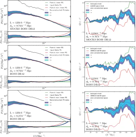
Figure 9. Left panels:power spectra of the reconstructed density fieldsδ(zref) on a mesh andright panels:quadrupoles of the galaxy distribution{sobs}and{r}based onupper panels: a light-cone mock (including survey geometry) withd
L= 9.76h−1Mpc, middle panels: the BOSS DR12 data withdL= 9.76h−1Mpc, andlower panels: the BOSS DR12 on withdL= 6.25h−1Mpc. Power spectra show the mean (dashed blue line) over 6000 samples with 1 and 2σcontours (light and dark blue shaded areas, respectively), as compared to the raw galaxy power spectrum (black solid line), the nonlinear (red solid line), and the linear power spectrum (green solid line) assuming the fiducial cosmology. Quadrupole correlation functions show the mean (dashed blue line) over 6000 samples (10 spaced samples in intervals from 500 iterations covering 4000 Gibbs-iterations for quadrupoles to reduce computations) with 1 and 2
σcontours (light and dark blue shaded areas, respectively), as compared to the raw galaxy power spectrum (black solid line), and the corresponding computations for the catalogues in real (green line for mocks only) and redshift space (red line).
for smoothing scales of aboutrS= 2h−1 Mpc. In fact for a smoothing scalerS between 1 and 2 h−1 Mpc one can po-tentially obtain unbiased results beyond k = 0.5hMpc−1. While our chains with 1283were run with velocities derived from density fields smoothed withrS = 7h−1 Mpc, our re-constructions with 2003 were run using rS = 2h−1 Mpc. This variety of smoothing scales serves us to test the ro-bustness of the velocity reconstructions depending on this parameter. In fact we manage to recover the monopoles in real space down to scales of aboutk∼0.2hMpc−1(see left
10-2 10-1
102
103
104
P
(
k
)[
M
pc
3
/h
3]
Planck linear PS Input Data PS Planck non-linear PS Reconstructed PS data
2σ 1σ
10-2 10-1
k
[
h
Mpc
−1]
0.5 0.0 0.5 1.0 1.5 2.0 2.5
P
(
k
)
/Plin
ea
r
(
k
)
L = 1250h−1Mpc
dL= 9.76h−1Mpc
BOSS DR12
with velocity dispersion
0 20 40 60 80 100 120 140 160
r[h−1Mpc]
−50
0 50 100
Q
(
r
)
·
r
2
real-space mock CMASS redshift-space
ARGOcorrected real-space
2σ
1σ
L = 1250h−1Mpc
dL= 9.76h−1Mpc
BOSS DR12
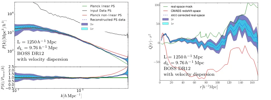
[image:13.595.82.549.50.223.2]with velocity dispersion
Figure 10.Same as Fig.9but including velocity dispersion.
reference. The upper right panel in Fig.9demonstrates that we cover the real space quadrupole down to scales of about
r∼20h−1Mpc. Deviations on large scales (∼>120h−1Mpc) between the recovered and the true quadrupoles are due to the large empty volume which pushes the solution to be closer to zero than in the actual mock catalogue. In fact, we showed in a previous paper that one can recover with this method the quadrupole features of the particular real-isation when considering complete volumes (Kitaura et al. 2016b). The results are consistent when comparing lower to higher resolution reconstructions (middle to lower right pan-els). However, we see that the uncertainty (shaded regions) in the quadrupole increases in the higher resolution case. This is expected as the coarser grid smooths the peculiar velocities and tends to underestimate them. In addition, we have run a reconstruction chain including velocity disper-sion, showing that this will also enhance the error bars in the quadrupole, however yielding the same qualitative re-sults as without that term (see lower panels in Fig.10). We observe a slightly enhanced uncertainty in the monopole and quadrupole on large scales. A proper treatment of the veloc-ity dispersion requires, however, at least a densveloc-ity dependent dispersion term, or even looking at the tidal field Eigenval-ues (see Kitaura et al. 2016b). This is however, computa-tionally more expensive and requires a number of additional parameters. We thus leave such an effort for later work. The accuracy of the quadrupole reconstruction presented in this paper seems to be superior than in some of the standard BAO reconstruction techniques (Vargas-Maga˜na et al. 2015; Burden et al. 2015), see in particular, right panel in Fig. 8 inKitaura et al.(2016a) showing the quadrupole after BAO reconstruction for a set of mock Multidark-patchy BOSS DR12 CMASS catalogues very similar to the ones used here. We note that while the monopoles of the dark matter field are trivially computed from the reconstructed samples on complete meshes, the computation of the quadrupoles of the galaxies needs more computational efforts to account for survey geometry and radial selection functions (see, e.g., Anderson et al. 2014a). Fig. 11 shows slices in the x−z
plane of the galaxy number counts, the completeness, and the reconstructed density fields. One can clearly recognise prominent features in the data in the reconstructed density
fields. It is remarkable however, how these features appear balanced without selection function effects, in such recon-structions. Only when one computes the mean over many realisations, one can see that larger significance in the recon-structions correlates with higher completeness values. The vanishing structures in unobserved regions further demon-strates the success in sampling from the posterior distribu-tion funcdistribu-tion. Fig. 12 shows that the lognormal fields are indeed reasonably Gaussian distributed in terms of the uni-variate probablity distribution function. In fact the absolute skewness is reduced from about 6.4 to less than 0.03 with means being always smaller than |hδLi| < 0.13 for differ-ent completeness regions. As we will analyse below the 3pt statistics does, however, not correspond to a Gaussian field.
4.3 The cosmic web from lognormal-Poisson reconstructions
So far we have been reconstructing the linear component of the density field in Eulerian space at a reference red-shift within the lognormal approximation. We can, however, get an estimate of the nonlinear cosmic web by performing structure formation within a comoving framework, i.e., with-out including the displacement of structures, as our recon-structed linear density fields already reside at the final Eule-rian coordinates. One can use cosmological perturbation the-ory to make such a mapping (seeKitaura & Angulo 2012). We will rely here on the classicalZel’dovich (1970) frame-work. By demanding mass conservation from Lagrangian to Eulerian spaceρ(q)dq=ρ(r)dr, we get an equation for the cosmic evolved density field within comoving coordinates: 1 +δPT(q) =J−1 (with the supercript standing for pertur-bation theory), whereJis the Jacobian matrix often called the tensor of deformation: Dij ≡ δijK+ Ψi,j(q, z). By
do-ing the proper diagonalisation one finds that the comovdo-ing evolved density field can be written as:
δPT(q, z) = 1
(1−D(z)λ1(q))(1−D(z)λ2(q))(1−D(z)λ3(q)) −1,
(44)
whereλiare the Eigenvalues of the deformation tensor with
4 2 0 2 4 0.00
0.05 0.10 0.15 0.20 0.25 0.30 0.35
mean w= 0 mean 0< w <= 0.2 mean 0.2< w <= 0.4 mean 0.4< w <= 0.6 mean 0.6< w <= 0.8 mean 0.8< w <= 1
δL
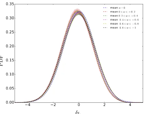
Figure 12.PDF of the matter statistics for different complete-ness values from 6000 reconstructions on a mesh of 2003and reso-lutiondL= 6.25h−1Mpc for the linear component reconstructed with the lognormal-Poisson model. The corresponding skewness range between−10−4and
−0.09 with means being always smaller than |hδLi|<0.13. The skewness is thus reduced by two orders of magnitude, as compared to a skewness of∼7 corresponding to the galaxy overdensity on a mesh with a cell resolution of 10h−1 Mpc.
over the formation of the cosmic web (seeHahn et al. 2007). In fact we could use the reconstructed velocity field to com-pute the shear tensor and study the cosmic web (Bond et al. 1996). We will however, focus on the largest Eigenvalue de-noting the direction of first collapse to form the filamentary cosmic web. We can Taylor expand the previous equation within the Eulerian framework yielding
δPT(r, z)'D(z)λ1(r) +λ+(r, z), (45) with λ+ being the higher order contributions including the rest of Eigenvalues, which can be approximated by
λ+(r, z)' −hD(z)λ
1(r)i. This expression avoids the prob-lem of formation of caustics, as present in Eq.44. We have tested other expansions including the rest of Eigenvalues, however, with less success in describing the nonlinear cos-mic web. The operation of retaining the information of the largest Eigenvalue can also be interpreted, as filtering out the noisy part of the Gaussian field. This technique could potentially be useful to effectively enhance the cosmic web of a low resolution simulation for mock catalogue production. We leave a more thorough investigation of other possible comoving structure formation descriptions for later work. Since this theory is based on the Gaussian density field, we will compute the Eigenvalues based on the linear com-ponent of the density field δL. In particular, we will com-pute them from the gravitational potential φL ≡ ∇−2δL, solving the Poisson equation with the inverse Laplacian op-erator in Fourier space, to obtain the correspoding tidal field tensor. By applying Eq. 45 we thus get the linear component of the gravitationally evolved density field in Eulerian space, which we will denote as δPTL (r). We now can compute the nonlinear component by doing the trans-formation δPT(r) = exp(δPTL (r) +µ(δ
PT
L (r))−1, having the physical meaninful property of yielding positive defi-nite density fields. To ensure that this field shares the same
power spectrum, as the lognormal reconstructed density field
δ(r) = exp(δL(r) +µ(δL(r)))−1, we apply in Fourier space
ˆ
δPTL ,f(k) =pPtrans(k) ˆδ PT L (k)
q
h|ˆδPT
L (k)|2i∆k
, (46)
where the nonlinear transformed power spectrumPtrans(k) is found iteratively. The ratio between the target power spectrum and the one obtained at a given iteration is multiplied to Ptrans(k) from the previous iteration until the nonlinear power spectra averaged in ∆k-shells coin-cideh|δˆPT,f(k)|2i∆
k' h|ˆδ(k)|2i∆k(i.e., the power spectrum
from the nonlinear transformed lognormal density field), in a givenk-range within a given accuracy. As a starting guess ofPtrans(k) we takeh|δˆL(k)|2i∆
k (i.e., the power spectrum
from the linear lognormal density field). In practice, less than 15 iterations are necessary to be accurate within bet-ter than 1% up to at least 70% of the Nyquist frequency using about 100 ∆k-bins for meshes of 2003cells on cubical volumes of 1250h−1 Mpc side, requiring less than 100son 8 cores. This operation is justified, as we are dealing with the Gaussian component of the density field, permitting us to
define a pseudo white noise ˆδPT L (k)/
q
h|ˆδPT
L (k)|2i∆k, which
Figure 13.Same as Fig.11, but for thex−yplane.
5 SUMMARY AND CONCLUSIONS
In this work, we have presented a Bayesian phase-space (density and velocity) reconstruction of the cosmic large-scale matter density and velocity field from the SDSS-III Baryon Oscillations Spectroscopic Survey Data Release 12 (BOSS DR12) CMASS galaxy clustering catalogue. We have
demonstrated that very simple models can yield accurate re-sults on scales larger thank∼0.2hMpc−1.
In particular we have used a set of simple assumptions. Let us list them here
Figure 14. Slices of the ensemble averaged Zeldovich transformed density field shown in Figs.11(left) and13(right) with another colour bar for visualisation purposes and the corresponding real space galaxy number count per cell overplotted in red.
Figure 15.Slices of the variance corresponding to the(left panel:)x−zplane, and(right panel:)x−yplane shown in Figs.11and 13, respectively.
• linear theory relates the peculiar velocity field to the density field,
• the volume is a fair sample, i.e. ensemble averages are equal to volume averages,
• cosmic evolution is modelled within linear theory with redshift dependent growth factors, growth rates, and bias,
• a power law bias, based on the linear bias multiplied by a correction factor, which can be derived from renormalised perturbation theory, relates the galaxy expected number counts to the underlying density field.
This has permitted us to reduce the number of parameters and derive them consistently from the data, with a given
smoothing scale and a particular ΛCDM cosmological pa-rameter set.
We have included a number of novel aspects in theargo code extending it to account for cosmic evolution in the linear regime. In particular, the Gibbs-scheme samples
• the density fields with a lognormal-Poisson model, • the mean fields of the lognormal renormalised priors for different completeness values,
• the number density normalisation at different redshift bins,
[image:17.595.52.560.316.541.2]• and the real space radial selection function from the reconstructed real space positions of galaxies (accounting for the “Kaiser-rocket” effect).
Our results show that we can get unbiased dark matter power spectra up tok∼0.2hMpc−1, and unbiased isotropic quadrupoles down to scales of about 20h−1 Mpc, being far superior to redshift space distortion corrections based on traditional BAO reconstruction techniques which start to deviate at scales below 60h−1 Mpc.
As a test case study we also analyse deviations of Pois-sonity in the likelihood, showing that the power in the monopole and the scatter in the quadrupoles is increased towards small scales.
The agreement between the reconstructions with mocks and BOSS data is remarkable. In fact, the identical algo-rithm with the same set-up and parameters were used for both mocks and observations. This confirms that the cos-mological parameters used in this study are already close to the true ones, the systematics are well under control, and gives further support to ΛCDM at least on scales of about 0.01<∼k <∼0.2hMpc−1.
We also found that the reconstructed velocities have a statistical correlation coefficient compared to the true ve-locities of each individual lightcone mock galaxy ofr∼0.7 including about 10% of satellite galaxies with virial mo-tions. The power spectra of the velocity divergence agree well with theoretical predictions up to k ∼ 0.2hMpc−1. This is far superior to the results obtained from simple lin-ear reconstructions of the peculiar velocities directly applied on the smoothed galaxy field for which statistical correla-tion coefficients of the order of 0.5 are obtained (Planck Collaboration et al. 2016, though this work used the Sloan main sample at lower redshifts being further in the nonlin-ear regime, making a direct comparison difficult). Improved results can be obtained with Wiener-filter based techniques, which need to correct for the bias in a post-processing way (Schaan et al. 2015). It would be interesting to compare the different methods, in particular considering that the en-semble average is not equal to the maximum of the poste-rior for non-Gaussian PDFs, as we consider here. Although it may seem surprising to get such accurate results from simply assuming linear theory to derive the peculiar mo-tions, we expect that linearised density fields as the ones ob-tained from lognormal-Poisson reconstructions (even if one takes the nonlinear transformed one), yield improved veloc-ity fields (see Falck et al. 2012; Kitaura & Angulo 2012). Also, while linear theory tends to overestimate the pecu-liar velocity field, the chosen grid resolution with the ad-ditional smoothing compensates for this yielding unbiased reconstructed peculiar motions. We have seen that for a given resolution the additonal Gaussian smoothing radius (and the cell resolution) can be derived from the velocity divergence power spectrum to match the linear power spec-trum in the quasi-linear regime (0.1∼<k <∼0.5hMpc−1). We demonstrated that the reconstructed linear component re-duces the skewness by two orders of magnitude with respect to the density directly derived from smoothing the galaxy field on the same scale.
We have furthermore demonstrated how to compute the Zeldovich density field from the lognormal reconstructed density fields based on the tidal field tensor in a
parame-ter free way. The recovered filamentary network remarkably connects the discrete distribution of galaxies. The real space density fields obtained in this work could be used to recover the initial conditions with techniques which rely on knowing the dark matter field at the final conditions (see e.g.Wang et al. 2013,2014).
We aim to improve the Bayesian galaxy distance esti-mates going to smaller scales, by using non-Poisson likeli-hoods and including a correction of the virialised motions (Ata et al. 2015;Kitaura et al. 2016b). One could also ex-plore other priors based on perturbation theory (e.g.Kitaura & Heß 2013;Heß et al. 2013).
Despite of the potential improvements to this work, the reconstructed density and peculiar velocity fields obtained here can already be used for a number of studies, such as BAO reconstructions, kinematic Sunyaev-Zeldovich (kSZ), integrated Sachs-Wolfe (ISW) measurements, or environ-mental studies.
ACKNOWLEDGMENTS
MA thanks the Friedrich-Ebert-Foundation for its support. MA and FSK thank Uros Seljak for the hospitality at LBNL and UC Berkeley and for enriching feedback, and the In-stituto de F´ısica Te´orica (IFT UAM-CSIC) in Madrid for its support via the Centro de Excelencia Severo Ochoa Program under Grant SEV-2012-0249. FSK also thanks Masaaki Yamato for support at LBNL and for encourag-ing discussions. CC acknowledges support from the Span-ish MICINNs Consolider-Ingenio 2010 Programme under grant MultiDark CSD2009-00064 and AYA2010-21231-C02-01 grant. CC were also supported by the Comunidad de Madrid under grant HEPHACOS S2009/ESP-1473. GY ac-knowledges financial support from MINECO (Spain) under research grants AYA2012-31101 and AYA2015-63810-P. The MultiDark Database used in this paper and the web ap-plication www.cosmosim.org/ providing online access to it were constructed as part of the activities of the German Astrophysical Virtual Observatory as result of a collabo-ration between the Leibniz-Institute for Astrophysics Pots-dam (AIP) and the Spanish MultiDark Consolider Project
CSD2009-00064.CosmoSim.org is hosted and maintained
by the Leibniz-Institute for Astrophysics Potsdam (AIP). The BigMultiDark simulations have been per-formed on the SuperMUC supercomputer at the Leibniz-Rechenzentrum (LRZ) in Munich, using the computing re-sources awarded to the PRACE project number 2012060963. Funding for SDSS-III has been provided by the Al-fred P. Sloan Foundation, the Participating Institutions, the National Science Foundation, and the U.S. Depart-ment of Energy Office of Science. The SDSS-III web site is http://www.sdss3.org/.