Provenance network analytics: an approach to data analytics using data provenance

https://doi.org/10.1007/s10618-017-0549-3

Provenance Network Analytics

An approach to data analytics using data provenance

Trung Dong Huynh1 · Mark Ebden2 · Joel Fischer3 · Stephen Roberts2 · Luc Moreau4

Received: 18 October 2016 / Accepted: 26 December 2017 © The Author(s) 2018. This article is an open access publication

Abstract Provenance network analytics is a novel data analytics approach that helps infer properties of data, such as quality or importance, from their provenance. Instead of analysing application data, which are typically domain-dependent, it analyses the data’s provenance as represented using the World Wide Web Consortium’s domain-agnostic PROV data model. Specifically, the approach proposes a number of network metrics for provenance data and applies established machine learning techniques over such metrics to build predictive models for some key properties of data. Applying this method to the provenance of real-world data from three different applications, we show that it can successfully identify the owners of provenance documents, assess the quality of crowdsourced data, and identify instructions from chat messages in an alternate-reality game with high levels of accuracy. By so doing, we demonstrate the different ways the proposed provenance network metrics can be used in analysing data, providing the foundation for provenance-based data analytics.

Keywords Data provenance·Data analytics·Network metrics·Graph classification

Responsible editor: Charu Aggarwal.

We gratefully acknowledge funding from the UK Engineering and Physical Sciences Research Council (EPSRC) for project ORCHID, Grant EP/I011587/1, and for Project SOCIAM, Grant EP/J017728/2. Data statement: The data used for the production of this article, along with the associated experiment code, is publicly available athttps://github.com/trungdong/datasets-provanalytics-dmkd.

B

1 _{Electronics and Computer Science, University of Southampton, Southampton, UK}

1 Introduction

Provenance, a description of what influenced the generation of a piece of information or data, has become an important topic in several communities since it exposes how information flows in systems, providing the means to make them accountable and helping users decide whether information is to be trusted (Moreau2010). Provenance has been recorded in an increasing number of applications, from legal notices,1climate science (Ma et al. 2014), medical applications,2 scientific workflows (Alper et al.

2013; Silva et al.2011; Davidson et al. 2007; Altintas et al.2006), computational reproducibility (Chirigati et al.2013), emergency response (Ramchurn et al.2016), and in the geospatial domain.3

As a provenance description ‘links’ artefacts with their influences, it can be represented in a graph, called aprovenance graph, whose nodes represent the arte-facts/influences and whose edges their relations with one another. Studying such graphs, e.g. by visualising them, can facilitate understanding of the provenance infor-mation they contain. However, in a typical application, provenance graphs can quickly become very large and complex; this makes it difficult to interpret their informa-tion manually. For instance, as an indicainforma-tion, the 2014 ediinforma-tion of the United States’ National Climate Assessment report4_{was published with full provenance information} linking its data and recommendations to 242 authors and over 500 distinct techni-cal inputs (Tilmes et al.2013). The scale is a few magnitudes larger with automated applications. CollabMap (Ramchurn et al.2013), an online crowd-sourcing platform, recorded more than 5000 provenance graphs over 3 months running, many of which contain 30–200 nodes, 50–700 edges. Scientific workflows (e.g. Wolstencroft et al.

2013; Silva et al.2011; Gil et al.2011; Bowers et al.2008) being applied to peta-scale problems, are also generating vast amount of provenance information. Such large and complex graphs are overwhelming for manual interpretation or verification (of data correctness, for instance). Therefore, an automated and principled way to analyse provenance data of such scales and, more importantly, to understand what they convey with respect to the data they describe, is much needed.

Against this background, in this paper, we proposeprovenance network analytics, a novel data analytics approach that combines network analysis and established machine learning techniques (Russell and Norvig2010, Ch. 18) over provenance information generated automatically from log and instrumentation of applications. It provides a generic way to analyse provenance information with the aim of revealing real-word characteristics of the data about which it describes. Our contributions to the state-of-the-art are as follows:

1. First, we adapt a number of existing network metrics (Newman 2010) to suit provenance graphs and define provenance-specific ones to summarise the

topo-1 _{https://www.thegazette.co.uk/.}

2 _{https://www.hl7.org/fhir/provenance.html.}

3 _{http://www.opengeospatial.org/projects/initiatives/ows-10.}

4 _{The online version of the report, provided with its provenance, is available athttp://nca2014.globalchange.}

logical structure of provenance graphs. Theprovenance network metrics can be computed in a generic manner from provenance records and are independent of domain-specific information. Therefore, they provide the basis for analysing and/or comparing provenance graphs quantitatively, even those from different applica-tions.

2. Second, we make use of the provenance network metrics to construct predictive models on provenance information based on known ground truths to relate prove-nance information with properties of data, such as their quality or importance. Once successfully trained for an application, those predictive models operate without relying on domain-specific information. By so doing, we devise a novel analytics method that analyses data using their provenance,notthe data themselves. Thanks to the generic nature of the proposed provenance network metrics, our approach can be used to study data, via the means of their provenance graphs, in applications where provenance information is recorded.

3. Finally, we report the successful application of the above method on the prove-nance of real-world data from three different applications: identifying owners of provenance documents, assessing the quality of crowd-generated data in Col-labMap, and identifying instructions from chat messages in an alternate-reality game. The applications were selected in part because they allow us to verify the accuracy of the proposed analytics via known ground truths or via an alternative method. In these applications, our analytic method achieved high levels of accu-racy classifying data based on the provenance of such data. By so doing, we also demonstratehowthe provenance network analytics approach can be concretely applied in specific contexts as a generic tool for data analytics.

The remainder of this paper is organised as follows. Section2introduces the prove-nance network metrics that serve as the basis for the proveprove-nance network analytics method presented in Sect.3. Section4describes the evaluation methodology. In Sect.5, we report on how the method was used to correctly identify owners of provenance graphs. Section6specialises the approach for quality assessment and demonstrates how the quality of crowd-generated data is classified. Section7shows that the same approach can help identify instructions from chat messages in the Radiation Response Game (Fischer et al.2014). We relate our approach to existing work in Sect.8 and conclude the paper with directions for future work in Sect.9.

2 Provenance network metrics

Fig. 1 The core PROV elements and relations. Adapted from Lebo et al. (2013)

influenced in some ways byagents. Such records can be packaged together into a

provenance documentfor the purpose of exchanging provenance information. Since provenance information describes how various elements were related to, or influenced by, one another, it can be viewed as a directed graph in which those elements (i.e. entities, activities, agents) are represented as nodes, and the relations between them (e.g. used, wasGeneratedBy, wasDerivedFrom) as directed edges. Such a graph is called aprovenance graph. Given that some provenance graphs can be very large, the challenge is how to extract useful information and knowledge from complex provenance graphs. In that respect, we turn to the established field of graph theory for principled methods to analyse graphs. Specifically, we are interested in network metrics that allow us to summarise the topological characteristics of a provenance graph, such as its shape, its size, or how its nodes tend to connect to one another. Such network metrics are generic and can be calculated on any graphs, including provenance ones. They provide us a way to summarise provenance graphs into a set of generic network features. As a result, they allow for the comparisons of provenance graphs, even those from different domains or applications, without the need for the knowledge required to interpret domain-specific information contained therein.

In the following sub-sections, we enumerate the network metrics we employ for our analysis of provenance graphs and provide their formal definitions. Section2.1

describes the generic network metrics which we adapted to work with provenance graphs. We then define provenance-specific network metrics in Sect.2.2to take advan-tage of provenance-specific information readily available in a provenance graph such as the types of nodes and the relations between them.

2.1 Generic network metrics

A provenance graph is a directed graphG =(VG,EG), with vertex setVGand edge set

EG. Vertices inVGrepresent the PROV elements (i.e. entities, activities, and agents). There is an edgee=vi, vj

that gives the provenance types of all vertices and edges in a provenance graph as follows:

ElementTypes= {Entity,Activity,Agent} (1) RelationTypes= {Generation,Usage,Start,End,Derivation,Invalidation,

Communication,Attribution,Association,Delegation, Membership,Alternate,Specialization,Influence}

(2)

type= (VG→ElementTypes)∪(EG→RelationTypes) (3)

In order to summarise the topological characteristics of a provenance graph, we adopt common existing network metrics for this. Those metrics regard a provenance graph as an ordinary directed graph and, therefore, disregard provenance-specific infor-mation (which, however, will be later considered in Sect.2.2). As a convention, the metrics in this section are defined on an input graphG=(VG,EG)and for the sake of brevity we omitGwhere it is unambiguous. The generic network metrics included in our analyses are:

– Number of nodesn = |V|, which is also the number of provenance elements in G.

– Number of edgese= |E|, which is also the number of provenance relations inG. – Graph diameterdGis the longestdistancein a graphG, where the distance between two verticesu andv is defined as the length of the shortest path between them, denoted byd(u, v). The graph diameter reflects how “spread out” the provenance graphGis.

dG = max

u,v∈VG

d(u, v) (4)

Since nodes in provenance graphs are separated by directed edges, thereby pre-venting some nodes from forming a path to certain others, strictly speaking, the diameter of each graph is, in many cases, infinite. However, by temporarily assum-ing the edges are undirected, we are able to calculate the diameter of a provenance graph. Hence, letGu =(V,Eu)be the undirected counterpart ofG, i.e. whose edges are the same as those inGbut undirected:Eu_{=E∪ {(v,u)|(u, v)∈E}.}

The diameter of a provenance graphG is then defined asdGu. For the sake of

brevity, we simply used to denote the graph diameter ofGu.

– Assortativity coefficientr: Assortativity, or assortative mixing, is the tendency for vertices in networks to be connected to other vertices that are like them in some way (Newman2003). The assortativity coefficient is the Pearson correlation coef-ficientr of degree between pairs of linked nodes. Positive values ofr indicate a correlation between nodes of similar degree, while negative values indicate rela-tionships between nodes of different degree.ris defined as per Eq. 24 in Newman (2003).

c_v= Γv

deg_vdeg_v−1 (5)

where deg_vis the number ofv’s neighbours andΓvis the number of edges between the neighbours. The averagecvof all vertices inGrepresents the extent of neigh-bourhood clustering in G. In order to avoid biased assessment of the metric, following Kaiser (2008), we exclude leaf and isolated nodes (i.e. deg_v 1) in our calculation:

ACC=C, whereC=c_v|v∈V∧deg_v>1 (6)

– Degree distribution: For many real-world graphs, the degree distribution follows a ‘power law’ such that the number of vertices Nk with degree k is given by

Nk ∝ k−α, whereα >0 is usually called the power-law exponent. We examine the degree distribution of an entire provenance graph to determine whether the distribution fits a power law as per the method of Clauset et al. (2009) and, if so, the degree-distribution power-law exponent (DPE). For provenance graphs whose degree distribution does not fit a power law andα is therefore undefined, we manually setα= −1.

2.2 Provenance-specific network metrics

In contrast to an ordinary directed graph, a provenance graph contains additional provenance type information on its the nodes and edges, as provided by the above type function (Eq.1). In this section, we extend generic network metrics to characterise provenance graphs while taking provenance types into account, and by so doing, define a set of provenance-specific network metrics:

– Numbers of entitiesne, activitiesna, and agentsnagin a provenance graph.

– Maximum finite distance (MFD): Since provenance relations represent a form of influence (Moreau and Missier2013), the length of the longest chain of influ-ence in a provenance graph is a useful characteristic of the graph. It can be viewed in the same vein as the graph diameter in the previous section but now on the directed graphG. In more detail, given two vertex sets X,Y ⊂ V, let

LX→Y the set of all finite distances separating a vertex inX with another inY: LX→Y = {d(u, v)|u∈ X∧v∈Y ∧d(u, v)= ∞}. The MFD between X and Y inG, denoted as mfdX→Y, is defined as follows:

mfdX→Y =

−1 ifLX→Y = ∅

maxLX_→Y otherwise

(7)

a provenance graph, we define nine different MFD metrics, one for each pair of node types: mfdts→te,ts,te ∈ {e,a,ag}, wheree,a, andagare our shorthand

notation to denoteV’s subsets whose elements areEntity,Activity, andAgent, respectively.

– MFD of derivations (mfdder): Since Derivation is the only influence relation

in PROV that has a strict time ordering (Cheney et al. 2013), we calculate additionally the MFD over this relation to examine the longest chain of deriva-tions in a provenance graph. For this, we consider Gder = (V,Eder), where

Eder = {e|e∈ E∧type(e)=Derivation}, i.e. the sub-graph that contains only

Derivationrelations fromG.

mfdder =

−1 ifEder = ∅

maxdG_der(u, v)|u, v∈V ∧dG_der(u, v)= ∞ otherwise (8)

where mfdderis set to−1 if there is no derivation relation in the graph.

– Average clustering coefficients by node type (ACCt): This is a variation of the

ACC metric (6); it is calculated from the local clustering coefficients of vertices of a given node typet∈ {e,a,ag}:

ACCt =Ct, whereCt =

c_v|v∈V∧type(v)=t∧deg_v>1 (9)

As there are three different provenance node types, there are also three provenance-specific ACC metrics:ACCe,ACCa, andACCag.

2.3 Summary

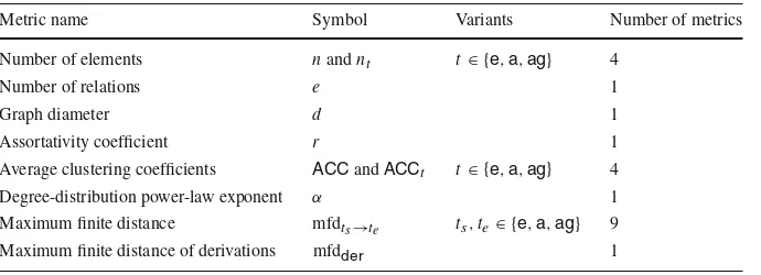
Combining the generic and provenance-specific network metrics (see Table1for a summary), for a given provenance graphG, its provenance network metricsP(G)are represented in a vector containing twenty-two elements:

Table 1 Glossary of provenance network metrics

Metric name Symbol Variants Number of metrics

Number of elements nandnt t∈ {e,a,ag} 4

Number of relations e 1

Graph diameter d 1

Assortativity coefficient r 1

Average clustering coefficients ACCandACCt t∈ {e,a,ag} 4

Degree-distribution power-law exponent α 1

Maximum finite distance mfdts→te ts,te∈ {e,a,ag} 9

P(G)= n, ne, na, nag, e, d,

r, ACC, ACCe, ACCa, ACCag, α,

mfde→e, mfde→a, mfde→ag, mfda→e,mfda→a,mfda→ag,

mfdag→e,mfdag→a,mfdag→ag,mfdder

(10)

In the next section, the above provenance network metrics serve as the basis for analysing provenance graphs to infer properties of the data they describe.

3 Provenance network analytics

The provenance network metrics defined in Sect.2can help us summarise a prove-nance graph’s topological characteristics and allow for the quantitative comparison of provenance graphs. The metrics can tell us a graph withn=4,e=3, andd =3 (i.e. a linear graph), for example, has a much different shape compared to a graph with

n = 4,e =3, andd = 2 (i.e. a star graph). However, without the ability to relate those values to domain-specific interpretation, say, the former is the result of a valid run while the latter is not, the network metrics alone would not help us to gain useful information contained in such graphs.

In this respect, we propose to apply existing supervised learning methods (see e.g. Russell and Norvig 2010, Ch. 18) to provenance graphs, using their network metrics as the features to predict some domain-specific characteristics of the data or events described by the graphs. The method requires a set of labelled training data, i.e. provenance graphs for which their classifications are known. The network metrics of those are then used as examples to train a predictive model for the interested classification. In essence, such a model predicts the label of awholeprovenance graph from its network metrics. If it can be shown that the model has a high predictive power given the training data, it can later be used for classifying unseen provenance graphs from the same domain. In more detail, the approach consists of three main phases:

– DesignThe purpose of this phase is to define the classification problem and to curate the required training data.

1. Define the classification labels: This step formalises the classification problem into a discrete set of labelsL. Given a piece of datax from the application domain, the classification problem becomes that of predicting the label ofx:

lx ∈ L. For example, if we want to determine whether an application run is valid or not, we could haveL = {valid,invalid}; if we want to assess the

quality of a data entity, we could haveL= {good,bad,uncertain}.

information (i.e. noise) that could confuse a learning algorithm. Some knowl-edge of the application domain is useful for this step. In the above example of application-run validity, for instance, one might choose the whole provenance graph recorded from one run as the input, while a much smaller graph covering the generation and usages of a data entity might be more appropriate for the assessment of its quality. Concrete examples of this step are later provided in Sects.5,6, and7, with the last showing how this step can be automated. 3. Curate training data: As this method relies on supervised learning techniques,

a curated set of labelled training dataS = {(x,lx)|lx ∈L}is required (i.e.lx

is defined for allxinS).

– TrainingHaving defined the label setL, defined the input provenance graphGx

for allxto be classified, and curated the training data setS, we build the predictive model which is, in essence, a function that mapsP(Gx)(Eq.10) toL:

1. Choose a supervised learning algorithm5that suitsLand the given data set. 2. Calculate the network metrics for the provenance graphs of the labelled data

and transform them into feature vectors with classification labels suitable as inputs to the chosen learning algorithm:I = {(P(Gx) ,lx)|(x,lx)∈S}.

3. Assess the accuracy of the learning algorithm on the input labelled data I. 4. If the accuracy in obtained in Step 3 is sufficiently high,6_{build the classifier}

forLfromIwith the chosen learning algorithm and proceed to the Prediction phase.

– PredictionUse the classifier from the Training phase to predict the labels of unseen data from their provenance.

4 Empirical evaluation

As a tool for data analytics, the provenance network analytics method aims to discover correlations between provenance information and properties of the data it describes. In order to demonstrate the approach, we apply the method to the provenance of real-world data from three different applications and report its performance in the following sections. Before doing that, however, we first describe the common methodology for evaluating the method.

Learning algorithm We use the CART (Breiman et al.1984) algorithm to train decision tree classifiers (specifically the Scikit-learn implementation by Pedregosa et al. 2011). Empirically, we find decision tree classifiers perform sufficiently well and were fast, although not always producing the highest accuracy. For the three selected applications, other learning algorithms we tested could only marginally improve classification accuracy while incurring significant increases in computing cost, in many cases several magnitudes higher, compared to that of the decision tree classifier (see the Extra 1 experiment in the online Supplementary Materials

5 _{Since the field of supervised learning is broad and it is not the focus of this paper, the reader is suggested to}

refer to Russell and Norvig (2010) and Marsland (2014) for an overview of the available learning algorithms and their suitability for a specific dataset.

for more details). In addition, a decision tree classifier is able to explain its clas-sification with decision rules, which may provide useful clues to understand the correlation between an application’s provenance data and the interested data prop-erties.

Balancing learning data To avoid producing biased classifiers, for datasets whose samples are unbalanced, we balance the input dataset I using the SMOTE method (Chawla et al.2011), which oversamples the minority samples such that each label has roughly the same number of samples inI.

Assessing accuracyIn order to benefit from all the available labelled data, which are small in some cases, we use 10-fold cross-validation (Kohavi1995). In particular, withIrandomly split into 10 equal subsets, we perform 10 rounds of learning; on each round a₁₀1 subset is held out as the test set and the remaining are used as training data. To further minimise the potential chance impact of random data splitting, we repeat the above cross-validation procedure 100 times, hence collecting 1000 accuracy scores in each experiment. We report the mean accuracy score alongside its 95% confidence interval in parentheses, for example, 98.13% (±0.01%).

In addition to the accuracy of classifiers, we also evaluate the following.

Relevance of metricsFrom each round of learning in the cross-validation proce-dure, the trained classifier automatically calculates the relevance of each input feature (i.e. each of the 22 network metrics in Eq.10) given the training data. In practice, this information will help us selectively reduce the number of metrics to be con-sidered within a specific application (if required). We report the three most relevant network metrics for each application, i.e. those with the highest average relevance values.

Generic versus provenance-specific metricsWe repeat the above process (i.e. the Training phase and evaluation) in two further experiments—one using only the generic network metrics (Sect.2.1) and the other only the provenance-specific network met-rics (Sect.2.2). Comparing the mean accuracy scores from the two experiments will help understand whether the network metrics based on provenance types bring added benefits to the classification application being discussed.

5 Application 1: Identifying owner of provenance documents

As the PROV data model provides a vocabulary for provenance information, it is likely that each provenance producer has its own “style” of writing provenance using the vocabulary. For example, a user or an application may produce provenance graphs with chains of derivations that can be long or short, with or without attributions to agents, etc. Such individual styles will manifest in different topological characteristics of the resulting graphs and, hence, differences in the graphs’ provenance network metrics. Our hypothesis is that the metrics could be used to identify the user or the application that produced a provenance graph. In order to verify this, we analyse the provenance network metrics of provenance documents deposited by the public at ProvStore, which is a public repository for provenance documents where a user can sign up for an account and store their provenance online for sharing or visualisation purposes (Huynh and Moreau2015). We apply the provenance network analytics method of Sect.3on those provenance documents to check how well it is able identify the documents’ owners, here used as a proxy for the application that generated the provenance. Note that those provenance graphs typically do not contain any information about the users who uploaded the graphs to ProvStore, so it is not possible to identify such users simply from querying the graphs.

5.1 Design phase

Graph labels We define the label setL = {u1,u2, . . . ,un}, wherelx = ui if the provenance documentxbelongs to userui andnis the total number of users.

Input graphsSince we want to identify the owner of a provenance graph based on its characteristics, we use the whole graph as the input graph, i.e.X =x.

Training dataIn order to upload a provenance document to ProvStore, the document’s owner needs to register for a user account there. As a result, the owner of each document on ProvStore is known and, hence, a curated labelled data set containing all those documents is readily available. Since each user owns a different number of documents, in order to ensure that there are sufficient samples to represent a user’s provenance documents the Training phase, we limit our experiment to users who have at least 20 documents. There are fourteen such users (the authors were excluded to avoid bias), who we named u1,u2, . . . ,u14; hence, there are 14 labels inL. Their numbers of documents range between 21 and 6,745, with the total number of documents in the data set is 13,870.

5.2 Training phase

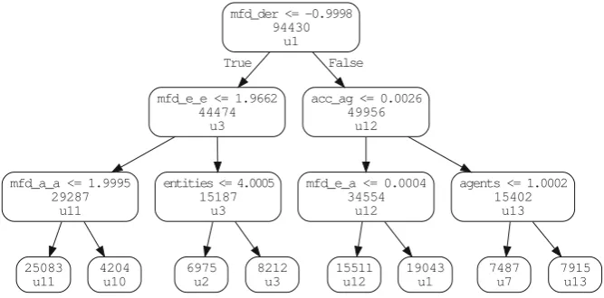
Fig. 2 The 3-depth decision tree for identifying owners of ProvStore documents

network metrics represents the “signature” of provenance graphs, reflecting how the user or application that produces them models and records provenance information.

5.3 Discussion

The above result confirms the predictive power of provenance network metrics in analysing and identifying provenance graphs. The classifier itself, however, is of limited utility since we already knew the owners of all documents on ProvStore. Having said that, this is not necessary the case in applications where provenance data come from multiple, potentially unreliable, sources. In such cases, the prove-nance network analytics method could potentially help identify strange or suspicious provenance traces for further investigation, akin to graph-based anomaly detec-tion techniques (Akoglu et al. 2015). For instance, as provenance traces reflect the behaviour of an actor, the method can detect behaviours that are significantly different from the typical, which might represent an intrusion in cyber security contexts.

After the Training phase, a decision tree classifier is able to explain its classification rules in the form of a decision tree. As an example, the decision tree for identifying document owners above is shown in Fig. 2, whose depth, however, was limited to three to fit the paper. From the decision tree, it is apparent that the most influential metrics selected by the algorithm are provenance-specific ones. The most important metrics, in this case, is mfdder; the tree splits the documents on ProvStore into two

subsets: ones without derivation relation (i.e. mfdder = −1, see Eq.8) and ones with at

least one derivation (the right branch). The tree shows the next most important metrics to distinguish provenance documents in this dataset are mfde→eandACCag. From

informed decision on which features that can safely be ignored (to save computation cost) in an automated manner, e.g. as per the method by Kohavi and John (1997).

In order to confirm that provenance type information indeed contributes into the above classification performance as suggested by the decision tree in Fig.2, we repeat the exercise, training a decision tree with the same dataset, but this time with only the six generic network metrics (i.e.n,e,d,r,ACC,α) and later only the provenance-specific metrics. Compared to the first experiment, which makes use of all the available network metrics, using only the generic metrics achieves a lower accuracy at 92.32% (±0.02%), while using only the provenance-specific metrics produces a similar accu-racy at 98.11% (±0.01%). These results suggest that provenance type information, as captured by the provenance-specific network metrics, indeed helps with identifying the originator of a provenance graph, and ignoring such information will result in a lower performance. Nevertheless, even with only six generic network metrics, the trained classifier still achieves a very high level of accuracy (92.32%). Therefore, we believe that characterising provenance information by their network metrics is a very promising approach, which can be effective even with a small set of metrics. In the next section, we develop this approach further to assess the usage of crowd-generated data to infer about their quality, using only their provenance information.

6 Application 2: Assessing the usage of crowdsourced data

The provenance of a piece of data tells us thehistorythat led to its creation. Analysing its provenance may help ascertain the data’s origin and that its production process was appropriate. It is, however, more challenging to infer about the data’s quality or signifi-cance from its history without knowing the quality, reliability, or trustworthiness of the data’s originator(s). Thus, instead of examining the data’shistoricalprovenance, we propose an alternative approach that examines the data’s “forward provenance”—the records of how the data is used following its creation (also captured in an application’s provenance traces). In this section, we apply the provenance network analytics on such “forward provenance” of crowdsourced data from CollabMap (Ramchurn et al.2013) to analyse their usage and, ultimately, their quality.

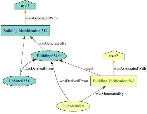
Fig. 3 A PROV graph from CollabMap

contributors to rate and correct each other’s contributions (i.e. buildings, routes, and route sets). They were, however, not allowed to verify their own work to avoid biases. In order to support auditing the quality of its data, the provenance of crowd activities in CollabMap was fully recorded: the data entities that were shown to users in each micro-task, the new entities generated therein, and their inter-relationships (see Fig.3

for a small example with two micro-tasks). In 2012, CollabMap was deployed to help map the area around the Fawley Oil refinery in the United Kingdom. It generated descriptions for 5,175 buildings, 4,997 routes, and 4,710 route sets. In this application, we apply the provenance network analytics method to construct three classifiers in order to assess the quality of CollabMap data from their provenance, one for each type of data.

6.1 Design phase

Graph labelsThe main aim of assessing the quality of CollabMap data is to determine which of them are sufficiently trustworthy to be included in the final evacuation map. For a data entityx, we wanted to know whetherx can be trusted to be correct (lx = trusted) or we are unsure about its quality (lx =uncertain). Thus, we define the label setL= {trusted,uncertain}.

x, we extract the provenance graph that contains all the activities and entities that were influenced byx. The intuition of the approach is similar to that of evaluating a publication from its citations. A highly cited academic paper, for example, is generally considered of high value thanks to its citations, or in other words, the relations it has with other papers. Such relations show how many times the paper was used in the generation of, or had an influence on, later papers.

Since a relation in PROV, i.e. an edge in our provenance graphs, represents some form of influence between its source and its target (Moreau and Missier2013), if there exists a path in a provenance graphGfrom nodevi to nodev0, denoted asvi −→∗ v0,

thenvi was, in some way, potentially influenced byv0. In other words, we consider

here the transitive (potential) influence of v0. It is possible to extract a sub-graph

DG_,x =(VG,x,EG,x)from graphGcontaining only the nodes that were directly or

indirectly influenced by a particular nodex, as follows:

VG_,x =

v∈V|v→∗ x

∪ {x} (11)

EG_,x =

e∈E|∃vs, vt ∈VG_,x(e=(vs, vt))

(12)

We call DG_,x thedependency graph of x extracted from the provenance graph G,

or the transitive closure ofx’s potential influence inG;VG_,xandEG,x are its vertex

set and edge set, respectively. Hence, it is now possible to analyse the influence of

xinGby examining the dependency graph DG_,x, which records howxwas used in

the application. Our hypothesis is that studying the dependency graph ofxwill reveal properties ofxsuch as its value or quality. Hence, in CollabMap, we use the dependency graph ofxas the input provenance graph in our quality analysis:X =DG_,x. Training dataFor the Training phase, we need to have a curated set of labelled training data. With the large amount of data generated in CollabMap, it was impractical to have them checked by experts. Collabmap instead relied on its participants to verify each other’s work: buildings, evacuation routes, and route sets were cross-checked by the participants multiple times. The validity of buildings, routes, and route sets was ascertained by giving those entities either positive or negative votes. From the votes recorded, following the TRAVOS trust model (Teacy et al.2006), we define the trustworthiness of an entityxbased on the beta family of probability density functions as follows:

τ (x)= α

α+β (13)

whereτ (x)is the trust value ofx (the mean of the beta distribution defined by the hyper-parametersαandβ) withα= p+1 andβ=n+1;pandnare the numbers of positive and negative votes ofx, respectively. Using the trust value 0< τ(x) <1, the labellx for any data entityxin CollabMap can now be assigned as follows:

lx =

trusted ifτ (a)0.75

uncertain otherwise (14)

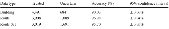
Table 2 CollabMap data quality classification results

Data type Trusted Uncertain Accuracy (%) 95% confidence interval

Building 4,491 684 90.03 ±0.06%

Route 3,908 1,089 96.98 ±0.04%

Route Set 3,019 1,691 95.70 ±0.05%

trust values of all buildings, routes, and route sets and assign them with corresponding labels as specified by Eq.14.

6.2 Training phase

We followed the methodology in Sect.4, using decision tree classifiers and the same training and evaluation process. In this application, we trained three classifiers to classify the quality of buildings, routes, and route sets, one for each CollabMap data type. The accuracy of the classifiers is presented in Table2with the 95% confidence intervals and the number of samples available for each data type. The results show that the classifiers trained on the provenance network metrics of dependency graphs predict the trust labels for buildings, routes and route sets in the test sets with a high level of accuracy: 90% for buildings, 97% for routes, and 96% and route sets.

6.3 Discussion

With such high accuracy levels achieved by the classifiers, it is important to note that our method did not rely on any domain-specific information from CollabMap but only on generic, domain-independent provenance network metrics. The strong correlation between the provenance network metrics and data quality in CollabMap discovered by the classifiers suggests that analysing network metrics of provenance graphs is a promising approach to making sense of the (real-world) activities and data they describe, such as classifying crowd-generated data into trust categories as in this case. The use of provenance network analytics in applications like CollabMap could potentially reduce significantly the number of required verification tasks (which incur a cost in resources and/or time). In such cases, only a much smaller set of verification tasks would need to be carried out to generate enough training data for building the quality classifiers as shown above. While the provenance of a piece of data is traditionally examined to study its history, the successful application of provenance network analytics over “forward provenance” to analyse data’s usage and significance in CollabMap shows that this can be an alternative useful approach for provenance analytics.

Fig. 4 The accuracy of quality classifiers for CollabMap buildings, routes, and route sets learned from generic and/or provenance-specific network metrics. Combining all the available metrics achieved the best classification accuracy

route sets. Such differences are understandable given that buildings, routes, and route sets were used differently to create new data in CollabMap. Although the decision trees and the most relevant metrics above do not explicitly account for the connec-tions between the features (i.e. the network metrics) and the prediction categories (i.e. the trust labels), they provide us with some starting points to help identify such connections in a later investigation.

Generic versus provenance-specific metricsWe retrained the three classifiers first using only the generic network metrics and later using only the provenance-specific metrics. The results (provided in Fig.4) show that the classifiers trained only on the generic network metrics performed better than those trained only on the provenance-specific metrics in classifying buildings and routes but not route sets. However, the highest accuracy in this application were achieved by making use of the full set of provenance network metrics across the three data types.

7 Application 3: Identifying instruction messages

In the previous application, we introduce a method to extract the dependency graph of an entity of interest from a bigger provenance graphs to analyse its usage after creation. In this section, we show how the method can be further optimised to achieve the highest classification performance, in this case, inferring the significance of a chat message in the Radiation Response Game (RRG) (Fischer et al.2014) from its “forward provenance”.

Fig. 5 Part of a PROV graph generated from a RRG capturing changes in one game activity

places as possible. Each field responder communicates with the headquarters and the others via a smart phone app. The app also tracks the actions taken by responders such as picking up, moving, and dropping off a target, in addition to their locations. In order to assist the analysis of team coordination in a RRG, we record what happened in a game in a provenance graph which contains the following information:

– Agents: the field responders participating in the game and the headquarters. – Entities: the targets and the messages communicated in the game.

– Activities: sending a message, picking up, transporting, and dropping off a target.

A small example of a RRG provenance graph is provided in Fig.5, which shows one game activity in whichAnimal121was picked up by two field responders, generating a new provenance entity,PickedUpAnimal121.1, which is its new version with the updated status. A RRG provenance graph describes all the activities in a RRG, and, hence, is a large graph,7covering the evolution of the whole game and how its players and targets changed over time.

Since RRG was designed to study team coordination, the communications among participants are of particular interest as they can reveal when teams are formed and what led to their formation. Therefore, in addition to automatically tracked game logs, each participant’s voice communication is also recorded by individual recorders and their actions captured by video cameras. In a typical RRG game, there are eight to ten audio streams (one per responder), and four video cameras capturing the actions of the headquarters and the field responders over 30 min. Hence, post-hoc analysis of these audio and video recordings to learn about when and how team coordination happened

requires significant human efforts. In practice, Fischer et al. (2014) relied on the chat messages as a source to identify when teaming decisions were made and where to focus their investigation in the audio and/or video recordings. In order to do so, they first manually classified the chat messages into a number of different categories, the most interesting being that ofdirectivesas their study aims to determine whether, when, and why an instruction is followed or rejected (Fischer et al.2014). Our intuition is that such instruction messages, either followed or rejected, would lead to various activities by the game’s participants following the moment the messages were received. For example, the participants could do as they were instructed, or they could send back more messages either to reject the instruction or to request further information. Since a RRG provenance graph also captures those activities, we believe that analysing the “forward provenance” of a chat message can help identify its role in the game. Hence, in what follows, we seek to apply the provenance network analytics method to identify instruction messages from their dependency (provenance) graphs.

7.1 Design phase

Graph labelsFor each message in a RRG, Fischer et al. (2014) classified them into one of the six categories: directives, assertives, expressives, declarations, commis-sives, and requests. Directives in RRG are typically instructions from the headquarters allocating tasks to the responder teams on the ground and are the targets for the clas-sifier. Therefore, we label a message withdirective, if it is one, orother, otherwise:

L= {directive,other}.

Input graphsThe dependency graph of a chat message in a RRG graph captures the activities that followed the message and, intuitively, is a suitable candidate to analyse to categorise a message. However, since a RRG graph evolves linearly along the time-line of a RRG, the size of such a dependency graph varies greatly depending on when in a game the message was sent; messages sent at the beginning of a game have significantly more (potential) dependants than those sent later in the game. In order to assess theimmediate“impact” of a message, we limit the dependency graph of a messagexto at mostkedges away from the message in a RRG provenance graph. We called such dependency graphD_Gk_,x =(V_Gk_,x,Ek_G,x)such that:

VGk_,x =

v∈V|v→k x

∪ {x} (15)

E_Gk_,x =

e∈E|∃vs, vt ∈VGk_,x(e=(vs, vt))

(16)

wherev→k xis true if there exists a path inGfromvtoxwhose length is at mostk. For a givenkand a messagex, we define the input graphX =Dk_G,x.

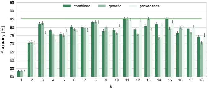
Fig. 6 The accuracy of the instruction message classifiers (of various dependency depthk) trained only on generic metrics, provenance-specific metrics, and both. The highest accuracy levels (marked by the horizontal line), 85%, were achieved with:k=11 (combined/generic/provenance),k=13 (generic), and

k=15 (combined). The accuracy level decreases withk>15

7.2 Training phase

We carried out the training phase for this application in a similar manner as in the two previous applications. The main difference is that dependency graphs of messages are parameterised byk, the depth of the dependency graphs to be analysed. In order to determine the optimal value ofkfor this application, we have the training carried out with different values ofk from 1 to 18.8 The cross validation procedure then informs us the value ofkthat yields the best classification performance for our intended application. At the same time, this provides us with an insight into how far the “impact” of a message could be in the whole RRG provenance graph. Thus, for eachk∈[1,18], we extractedDk_G,xfor each message, and calculated the provenance network metrics for it. We then proceed with the training of a classifier to predict the label of a message

xfrom its dependency graph. The mean accuracy of the classifier at each value ofk

and the confidence interval are plotted in Fig.6.

The results show that the classifier correctly identified directive messages on an average three out of four times fork≥3. It performed slightly worse atk=2 and did no better than the base line atk=1, suggesting that little or no useful network infor-mation was contained in such shallow dependency graphs. The exploration procedure discovers thatk=11 yields the top performance at 85.13% (±0.79%).

7.3 Discussion

In this application, we show how dependency graphs can be parameterised by their maximum depth (k) to help extract relevant input graphs for network analytics (in applications whose provenance graphs are too large and encompassing). The optimal value ofk can be discovered in an automated manner by trialling different values

and checking the classifier’s performance with each value as shown earlier. Although the message classifier’s accuracy is not as high as in the previous two applications, this level of accuracy (i.e. 85%) is sufficiently high for it to be useful as an automated analytic tool for the RRG study. It could assist post-hoc analysis of future RRG studies by labelling instructions from chat messages based on their provenance, significantly reducing manual efforts in classifying them as it has hitherto been done. Since our analytics method does not rely on the domain data but only on the provenance of activities in an RRG game, it can certainly be applied in other studies where similar provenance is captured. In those cases, the method can help identify points of interest in a study for further investigations, saving time and efforts of researchers going through voice and video recordings. In scenarios where instructions are already identified (e.g. tasks allocation, military orders), the result from this application suggests that analysing the “forward provenance” of such instructions could help determine their compliance with a predictive model.

Relevance of metricsAs with the previous applications, we examine the relevance of the network metrics; however, given the numerous configurations ofk, we only give a summary of the results here. The detailed results are available in the Supplementary Material. Across various values ofk, we found that the most influential metrics was the number of edgese, followed by the number of entitiesne and mfde→a. This is

compatible with our earlier intuition that a directive message generally would generate more game activities, manifesting in more entities and provenance relations (i.e. edges) in the message’s dependency graphs.

Generic versus provenance-specific metricsComparing the accuracy of classifiers trained only on the generic network metrics and that of those trained only on the provenance-specific metrics across the 18 values ofk, the result is mixed. As shown in Fig.6, both perform similarly in 7 cases, using provenance-specific metrics out-performs using only generic metrics in 7 cases, and in the remaining 4 cases, the reverse is true. It is difficult to draw a clear-cut conclusion from this. However, the result indicates that the provenance-specific metrics still plays a significant role in this application. Finally, both types of network metrics perform equally well in with

k=11, delivering the top accuracy for this application.

8 Related work

to changes in the relationships among sports players and coaches) rather than node attributes (namely a player’s performance statistics).

The field is continually evolving, and graphs can be viewed in a growing number of ways; provenance data itself can be interpreted as collaboration networks (Altintas et al.2010) or otherwise. Recently, Margo and Smogor (2010) examined a provenance graph based on components of a file-store, to show that provenance and other meta-data can successfully predict semantic attributes: in particular, they predicted file extensions in a file-history graph. (As in earlier sections, ‘predict’ refers not to the temporal sense of the word, but to the re-inferring of removed data.) Although their particular choice of attribute to predict “has few applications”, the study functioned as a useful proof of concept. The authors employed the C4.5 decision tree algorithm on their provenance graph, with the network structure and artefact attributes as input; the levels of accuracy achieved were comparable to our own, even though in the present work we examine provenance graphs of a different topology and size. The authors recognised that further exploration of the feature space over provenance graphs was called for; among other things, our methodology extends the types of features used in such analyses.

Similar to our data quality assessment in Application 2 (Sect.6), Ceolin et al. (2014) sought to assess trustworthiness of crowdsourced data using provenance information. They relied, however, on node attributes (such as timestamps and typing speeds) rather than the network topology, in a different application area to ours (annotation of museum collections), achieving accuracies of approximately 80%. CrowdTruth (Inel et al.2014) is another crowdsourcing annotation application that sought to derive the quality crowdsourced data from a set of metrics on disagreements within the collected data. This work derived the metrics from the actual content of the data, not from analysing the relationships between them as per our method.

Our method provides a broader type of analysis than certain previous work on hyperlink network analysis (Park2003) in which the links between web pages were studied to estimate the value of websites (e.g. their credibility) or to identify social networks. In the former case, the previous work only counted the number of links and did not investigate the network connections further than one link away (in contrast with the size of dependency graphs in our analyses). In the latter, the focus was on clustering similar nodes or detecting outliers, e.g. isolated nodes or those with few links, not on predicting node attributes as in this work. Also relatedly, Varlamis and Louta (2009) count network links in order to express trustworthiness, as an example application of the principle described by Yu and Singh (2000) that propagation can be considered one of the properties of trust (along with symmetry, transitivity, self-reinforcement, etc.) However, Varlamis and Louta (2009) did not have voting data available in order to assess the accuracy of their model in the way we could as in the CollabMap application.

More generally speaking, graphs, as a generic and flexible data representation, are ubiquitous in describing computation. Analysing graph data is, hence, an active research topic of multiple communities in a variety of fields such as graph-based semi-supervised learning (Subramanya and Talukdar2014), graph mining (Aggarwal and Wang2010), and more. The latter includes frequent pattern mining (Cheng et al.

2014), graph clustering (Gaertler2005), graph classification (Tsuda and Saigo2010), etc. Our work largely falls into the last area by providing a method for predicting the label of awholeprovenance graph, as opposed to predicting the label of a node in the graph, also known as “label propagation” (Bengio et al.2006). However, compared to other graph classification techniques, our method makes use of network metrics instead of graph kernels (Vishwanathan et al.2010) or boosting (Saigo et al.2009); and the metrics were specifically constructed to work with PROV provenance graphs. Such provenance network metrics have not been studied before and our work is the first to propose employing them for characterising real-world properties of data in an automated manner.

9 Conclusions

it instead relies on the opinions of the participants (e.g. via a voting-like mechanism). In this work, we propose applying machine learning techniques on the network met-rics of provenance graphs to explore and automate data characterisation. In particular, we have presented a generic and principled data analytics method for analysing data and applications based on their provenance graphs. Using this method, via the means of off-the-shelf machine learning algorithms, it is now possible to explore and learn about some properties of the data from their provenance in an automated manner. Since the method employs common network analyses and machine learning techniques on generic provenance graphs, it can be used in a wide range of applications where prove-nance are captured (or can be generated from application data/logs). Indeed, we have demonstrated the applicability of this method within three different applications: (1) identifying the owners of provenance documents on ProvStore, (2) classifying the trust labels for buildings, routes, and route sets drawn by crowd contributors in CollabMap, and (3) identify instructions from chat messages in the RRG; all resulted with high levels of accuracy. At the same time, we show how the method can be customised and optimised to suit a particular application context. Particularly, the results of Applica-tion 3 (Sect.7) also led us to believe that the provenance network analytics method can be a useful analytic tool for studying human activities or determining their compliance. The twenty-two provenance network metrics we propose as features for analysing provenance information (Sect.2) were chosen as the starting points of our investigation in this work. Although all of them were shown to contribute to the classification performance in the selected applications, each classification problem may still work well with a small subset of the metrics. Therefore, the relevance analysis is essential to identify those and to reduce the computation cost for unnecessary metrics. We plan to refine and develop further metrics from those twenty-two starting metrics. In particular, we are interested in refining the provenance-specific metrics to take into account the provenance semantics ofAlternateandSpecializationrelations, which convey a different kind of influence than the others.

While avoiding using domain-specific information allows the provenance network metrics to be generically applied, we also appreciate the potential value of application-specific data in improving classification performance. In addition, certain applications may produce provenance graphs having the same topological characteristics, resulting the same set of network metrics values, confusing predictive models based solely on those. Therefore, in another future direction, we plan to extend our proposed met-rics to utilise domain-specific information recorded in provenance information. We expect such customised provenance network metrics, albeit no longer generic, will help improve accuracy in analysing an application’s data and will work with provenance graphs of highly similar topology.

models of imperfect provenance information and their effects on provenance network analytics.

With an increasing number of applications continuously generating provenance,9 we can quickly get overwhelmed with torrents of provenance data requiring our atten-tion. The provenance network analytics method presented here can potentially be applied on provenance graph summaries, such as those produced by graph summari-sation techniques (e.g. Moreau2015; Riondato et al.2016), as significantly smaller proxies of the original provenance graphs, in order to lower computation costs. The analyses can also be extended to study the provenance network metrics that charac-terise the evolution of provenance graphs (like those introduced by Ebden et al.2012), which reflect the development of the tasks they represent. Such an extension could help us to understand developing dynamic behaviours, and to allow for appropriate on-the-fly interventions (in order to stop an undesirable behaviour from progressing, for instance).

In a wider context, provenance graphs do not only describe the origin of data, but they also reveal the interactions of agents in connected activities and how the activities themselves unfolded at the same time. The provenance network metrics presented in this work, therefore, could find useful applications in other areas in addition to those presented here. Analysing the influence of agents in the provenance graph of a collaborative task could identify the most valuable team member. Studying the distances between the agents in the graph could reveal close collaboration or team breakdown; or finding frequent patterns (Kuramochi and Karypis 2005; Yan et al.

2008) in provenance graphs may show how they usually work together. In addition, focusing on the activities in a graph could help detect bottlenecks, important data, and activities that were crucial to the outcome of a task. Given the generic nature of network analysis techniques, the possibilities are highly promising and vast.

Open Access This article is distributed under the terms of the Creative Commons Attribution 4.0 Interna-tional License (http://creativecommons.org/licenses/by/4.0/), which permits unrestricted use, distribution, and reproduction in any medium, provided you give appropriate credit to the original author(s) and the source, provide a link to the Creative Commons license, and indicate if changes were made.

A Supplementary Materials

In order to help reproduce the results shown in this paper, we publish the datasets and the code used in the experiments reported above in the (electronic) Supplementary Materials, whoseREADME.mdfile provides the full descriptions of the datasets and the code. In addition, the Supplementary Materials are also available online athttps:// github.com/trungdong/datasets-provanalytics-dmkd, where future updates and errata to the materials will be made.

References

Aggarwal CC, Wang H (2010) Graph data management and mining: a survey of algorithms and applications. In: Aggarwal CC, Wang H (eds) Managing and mining graph data, advances in database systems, chap 2, vol 40. Springer, Boston, pp 13–68.https://doi.org/10.1007/978-1-4419-6045-0_2

Akoglu L, Tong H, Koutra D (2015) Graph based anomaly detection and description: a survey. Data Min Knowl Discov 29(3):626–688.https://doi.org/10.1007/s10618-014-0365-y

Alper P, Belhajjame K, Goble CA, Karagoz P (2013) Enhancing and abstracting scientific workflow prove-nance for data publishing. In: Proceedings of the joint EDBT/ICDT 2013 workshops, ACM, New York, NY, USA, EDBT’13, pp 313–318.https://doi.org/10.1145/2457317.2457370

Altintas I, Barney O, Jaeger-Frank E (2006) Provenance collection support in the Kepler scientific workflow system. In: Proceedings of the 2006 international conference on provenance and annotation of data, Springer, IPAW’06, pp 118–132.https://doi.org/10.1007/11890850_14

Altintas I, Anand MK, Crawl D, Bowers S, Belloum A, Missier P, Ludäscher B, Goble CA, Sloot PMA (2010) Understanding collaborative studies through interoperable workflow provenance. In: McGuinness DL, Michaelis JR, Moreau L (eds) Provenance and annotation of data and processes. Springer, Berlin, Heidelberg, pp 42–58

Bengio Y, Delalleau O, Roux NL (2006) Label propagation and quadratic criterion. In: Olivier C, Schölkopf B, Zien A (eds) Semi-supervised learning. MIT Press, Cambridge, pp 193–216.https://doi.org/10. 7551/mitpress/9780262033589.003.0011

Bowers S, McPhillips T, Riddle S, Anand MK, Ludäscher B (2008) Kepler/pPOD: Scientific workflow and provenance support for assembling the tree of life. In: Freire J, Koop D, Moreau L (eds) Provenance and annotation of data and processes, Lecture Notes in Computer Science, chap 9, vol 5272. Springer, Berlin, pp 70–77.https://doi.org/10.1007/978-3-540-89965-5_9

Brandes U, Erlebach T (2005) Network analysis: methodological foundations. Springer, Berlin

Breiman L, Friedman J, Olshen R, Stone C (1984) Classification and regression trees. Wadsworth, Belmont Ceolin D, Nottamkandath A, Fokkink W (2014) Efficient semi-automated assessment of annotations

trust-worthiness. J Trust Manag 1(3):1–31.https://doi.org/10.1186/2196-064X-1-3

Chawla NV, Bowyer KW, Hall LO, Kegelmeyer WP (2011) SMOTE: Synthetic minority over-sampling technique. J Artif Intell Res 16:321–357.https://doi.org/10.1613/jair.953

Cheah YW, Plale B (2012) Provenance analysis: towards quality provenance. In: 2012 IEEE 8th international conference on e-science, IEEE, pp 1–8.https://doi.org/10.1109/eScience.2012.6404480

Chen P, Plale B, Aktas MS (2014) Temporal representation for mining scientific data provenance. Future Gener Comput Syst 36:363–378.https://doi.org/10.1016/j.future.2013.09.032

Cheney J, Perera R (2015) An analytical survey of provenance sanitization. In: Ludäscher B, Plale B (eds) Provenance and annotation of data and processes. IPAW 2014, Lecture Notes in Computer Science, vol 8628. Springer, Cham, pp 113–126.https://doi.org/10.1007/978-3-319-16462-5_9

Cheney J, Missier P, Moreau L, Nies TD (2013) Constraints of the PROV data model. W3C recommendation REC-prov-constraints-20130430, World Wide Web Consortium, http://www.w3.org/TR/2013/REC-prov-constraints-20130430/

Cheng H, Yan X, Han J (2014) Mining graph patterns. In: Aggarwal CC, Han J (eds) Frequent pattern mining, chap 13. Springer, Berlin, pp 307–338.https://doi.org/10.1007/978-3-319-07821-2_13 Chirigati F, Shasha D, Freire J (2013) Reprozip: using provenance to support computational

reproducibil-ity. In: Proceedings of the 5th USENIX conference on theory and practice of provenance, USENIX Association, Berkeley, CA, USA

Clauset A, Shalizi C, Newman M (2009) Power-law distributions in empirical data. SIAM Rev 51:661–703 Danger R, Curcin V, Missier P, Bryans J (2015) Access control and view generation for provenance graphs.

Future Gener Comput Syst 49:8–27.https://doi.org/10.1016/j.future.2015.01.014

Davidson SB, Boulakia SC, Eyal A, Ludäscher B, McPhillips TM, Bowers S, Anand MK, Freire J (2007) Provenance in scientific workflow systems. Data Eng Bull 30(4):44–50

Ebden M, Huynh TD, Moreau L, Ramchurn S, Roberts S (2012) Network analysis on provenance graphs from a crowdsourcing application. In: Groth P, Frew J (eds) Provenance and annotation of data and processes, Lecture Notes in Computer Science, vol 7525. Springer, Berlin, pp 168–182.https://doi. org/10.1007/978-3-642-34222-6_13

Martin D, Conein B (eds) COOP 2014—Proceedings of the 11th international conference on the design of cooperative systems. Springer, Nice, pp 49–67.https://doi.org/10.1007/978-3-319-06498-7_4 Gaertler M (2005) Clustering. In: Brandes U, Erlebach T (eds) Network analysis, Lecture Notes in Computer

Science, chap 8, vol 3418. Springer, Berlin, pp 178–215. https://doi.org/10.1007/978-3-540-31955-9_8

Gil Y, Ratnakar V, Kim J, Gonzalez-Calero P, Groth P, Moody J, Deelman E (2011) Wings: intelligent workflow-based design of computational experiments. IEEE Intell Syst 26(1):62–72.https://doi.org/ 10.1109/MIS.2010.9

Hussein J, Sassone V, Moreau L (2016) A template-based graph transformation system for the prov data model. In: Seventh international workshop on graph computation models GCM 2016

Huynh TD, Moreau L (2015) ProvStore: a public provenance repository. In: Ludäscher B, Plale B (eds) 5th international provenance and annotation workshop, IPAW 2014, Lecture Notes in Computer Science, vol 8628. Springer, Cologne, pp 275–277.https://doi.org/10.1007/978-3-319-16462-5_32 Inel O, Khamkham K, Cristea T, Dumitrache A (2014) CrowdTruth: machine-human computation

frame-work for harnessing disagreement in gathering annotated data. In: Mika P, Tudorache T, Bernstein A, Welty C, Knoblock C, Vrandeˇci´c D, Groth P, Noy N, Janowicz K, Goble C (eds) The semantic web— ISWC 2014, Lecture Notes in Computer Science, vol 8797. Springer, Berlin, pp 486–504.https://doi. org/10.1007/978-3-319-11915-1

Kaiser M (2008) Mean clustering coefficients: the role of isolated nodes and leafs on clustering measures for small-world networks. New J Phys 10(8):083,042.https://doi.org/10.1088/1367-2630/10/8/083042 Kohavi R (1995) A study of cross-validation and bootstrap for accuracy estimation and model selection.

In: Proceedings of the 14th international joint conference on artificial intelligence, vol 2. Morgan Kaufmann Publishers Inc., San Francisco, CA, USA, pp 1137–1143

Kohavi R, John GH (1997) Wrappers for feature subset selection. Artif Intell 97(1–2):273–324.https://doi. org/10.1016/S0004-3702(97)00043-X

Kolaczyk E (2009) Statistical analysis of network data. Springer, Berlin

Kuramochi M, Karypis G (2005) Finding frequent patterns in a large sparse graph. Data Min Knowl Discov 11(3):243–271.https://doi.org/10.1007/s10618-005-0003-9

Lebo T, Sahoo S, McGuinness D (2013) PROV-O: the PROV ontology. Tech. Rep. REC-prov-o-20130430, World Wide Web Consortium.https://www.w3.org/TR/2013/REC-prov-o-20130430/, W3C Recom-mendation

Ma X, Fox P, Tilmes C, Jacobs K, Waple A (2014) Capturing provenance of global change information. Nat Clim Change 4(6):409–413.https://doi.org/10.1038/nclimate2141

Margo D, Smogor R (2010) Using provenance to extract semantic file attributes. In: Proceedings of the 2nd conference on theory and practice of provenance, Berkeley, USA, USENIX Association

Marsland S (2014) Machine learning: an algorithmic perspective. Chapman and Hall/CRC, London Missier P, Bryans J, Gamble C, Curcin V, Danger R (2015) ProvAbs: Model, policy, and tooling for

abstracting prov graphs. Provenance and annotation of data and processes. IPAW 2014, Lecture Notes in Computer Science, vol 8628. Springer, Cham, pp 3–15. https://doi.org/10.1007/978-3-319-16462-5_1

Moreau L (2010) The foundations for provenance on the web. Found Trends Web Sci 2(2—-3):99–241. https://doi.org/10.1561/1800000010

Moreau L (2015) Aggregation by provenance types: a technique for summarising provenance graphs. In: Graphs as models 2015, London, UK, pp 129–144.https://doi.org/10.4204/EPTCS.181.9

Moreau L, Missier P (2013) PROV-DM: The PROV data model. Tech. Rep. REC-prov-dm-20130430, World Wide Web Consortium.http://www.w3.org/TR/2013/REC-prov-dm-20130430/, W3C Rec-ommendation

Moreau L, Clifford B, Freire J, Futrelle J, Gil Y, Groth P, Kwasnikowska N, Miles S, Missier P, Myers J, Plale B, Simmhan Y, Stephan E, Van den Bussche J (2011) The open provenance model core specification (v1.1). Future Gener Comput Syst 27(6):743–756.https://doi.org/10.1016/j.future.2010.07.005 Newman M (2010) Networks: an introduction. Oxford University Press, Oxford

Newman MEJ (2003) Mixing patterns in networks. Phys Rev E 67(2):026,126.https://doi.org/10.1103/ PhysRevE.67.026126