Parallel Behavior Composition for Manufacturing
Paolo Felli
University of Nottingham, UK
[email protected]
Brian Logan
University of Nottingham, UK
[email protected]
Sebastian Sardina
RMIT University, Australia
[email protected]
Abstract
A key problem in the manufacture of highly-customized products is the synthesis of controllers able to manufacture any instance of a given prod-uct type on a given prodprod-uction or assembly line. In this paper, we extend classical AI behavior compo-sition to manufacturing settings. We first introduce a novel solution concept for manufacturing com-position,target production processes, that are able to manufacture multiple instances of a product si-multaneously in a given production plant. We then propose a technique for synthesizing the largest tar-get production process, totar-gether with an associated controller for the machines in the plant.
1
Introduction
Manufacturing companies are increasingly faced with de-mands for variable volumes of high quality customised prod-ucts, produced rapidly and at low cost [Foresight, 2013]. One way of meeting such demands is through increased automa-tion, and in particular allowing production control software greater autonomy in determining how products will be ufactured. The application of autonomous systems in man-ufacturing has the potential to increase productivity, flexibil-ity and reliabilflexibil-ity, add value, and compensate for an ageing skilled workforce. However, the complexity of such “au-tonomous manufacturing systems” has so far prevented their widespread adoption. A key challenge in realising the po-tential of autonomous manufacturing is moving from human-authoring of the production control software that specifies how a particular product should be made, to theautomated synthesis of controllers that are able to manufacture any in-stance of a given product type on a particular production or assembly line.
The problem of synthesising complex (virtual) systems from simple existing modules has been addressed in AI, where it is referred to as the behavior composition prob-lem [De Giacomo et al., 2013]. The composition task in-volves synthesizing a controller to coordinate a set of avail-able behavior modules (e.g., automatic lights or blinds, TVs, microwaves, etc.) so as to implement a novel target behav-ior module (e.g., a smart house system). Standard behavbehav-ior
composition assumes a single sequential execution of the tar-get behavior module. While adequate for domains such as web-services [Calvaneseet al., 2008], these approaches are not applicable to the manufacturing domain.
In manufacturing, the target represents a process specified by a production recipe, which lists the steps necessary to manufacture items of a particular product type, and the or-der in which those steps should be executed. The recipe en-compasses all variations of the product type, e.g., variations in size, color or material, and decisions about how a particu-lar item should be manufactured are made at run-time, based on order information associated with the item, e.g., whether the item is to be blue or green. The steps in a recipe are en-acted byproduction resources, e.g., welding machines, paint-ing machines, etc. For example, in garment manufacture, a production recipe may specify how to make shirts of vari-ous colors and sizes, and the production resources may be fabric cutting, sewing and pressing machines. In general, a recipe consists of multiple steps, and (depending on avail-able production resources) it is often possible to start work on manufacturing another item before the items currently being manufactured have been completed. The aim is to construct atarget production processthat allows many instances of a product type (ideally as many as possible) to be produced at the same time on the available production resources. Criti-cally, such a process must allowallvariations of the product type specified by the recipe for each instance produced, as the specification of each item (e.g., whether it will be blue or green) is only known at run-time.
In this paper, we extend behavior composition [De Gia-comoet al., 2013; Stroeder and Pagnucco, 2009; Lustig and Vardi, 2009] to manufacturing settings. We formalise both production recipes and production resources, and propose a technique for synthesizing a target production process and controller capable of orchestrating the behaviors of the pro-duction resources to produce multiple instances of a product type in accordance with the recipe. To the best of our knowl-edge, our work is the first to consider the synthesis of con-trollers for multiple concurrent instances of a target process.
2
Production Recipes and Cycles
manufac-A X Y Z
α β
γ
R
A α X
β, γ
LR
Figure 1: A simple product recipeRand its production cycle.
ture any instance (e.g., a blue shirt of size XL) of a particular product type (e.g., shirts).
Definition 1. A production recipe is a tuple R = (L, l0, A, λR, F)where(i)Lis finite set of states andl0∈L
is the initial state;(ii) Ais a finite set of actions;(iii) λR ∶
L×A → L is an acyclic transition function with all final
states being sink states;(iii)F⊆Lis the set of final states.∎
A production recipe may be arbitrarily large and include options for which action to perform in a state that encode the different ways in which a product can be manufactured (e.g., due to variations within a product type). For example, once the fabric of a shirt has been cut, it may be dyed green, red, or blue: which color should be used for a particular product item is decided at run-time and is outside the model (e.g., by a human operator, or determined by information carried by the item itself, e.g., in the form of a radio-frequency identifi-cation (RFID) tag specifying the color). If a recipe is action-deterministic, i.e., only one action is available in each state of
R, this indicates that there is only one possible way of
man-ufacturing the product type.
We assume that recipes are acyclic and “terminating”: the manufacture of every product item requires a bounded num-ber of steps.1 For example, producing an item of the product type specified by the recipeRdepicted in Figure 1 requires
performing operationα(e.g., cut fabric) followed by either actionβ (e.g., dye blue) orγ (e.g., dye green), after which the item is deemed manufactured (statesYandZare final). Hence Rspecifies two different manufacturing alternatives
or product variations. As explained above, whether β or γ
will be performed for a particular item is decided at run-time, externally to the recipe.
While recipes specify how oneitem of a product type is to be manufactured to completion, a production plant aims to manufacture many instances of a product simultaneously, over and over, in principle forever. This continuous process is captured through the notion of production cycle.
Definition 2. Given a product recipeR = (L, l0, A, λR, F),
the production cycle induced by Ris a tuple LR = (L∖
F, l0, A, λ)such that λ(l) = λR(l)for all l ∈ L∖F, and
λ(l) =l0for eachl∈F. ∎
Intuitively, a production cycle represents the repeated exe-cution of a recipe. To represent the completion of one item and the beginning of the next item of the product type, we add a transition from the final states to the initial state of the recipe. When an item “returns” to the initial state (through a
1
It is straightforward to add constructs specifying the bounded repetition of a subprocess, e.g., to model the re-trying of a process (clean subprocess) until success (product sensed clean), and exiting after some number of repetitions (discard product).
sequence of transitions within its production cycle), it is con-sidered as “completed,” and the cycle can be “restarted” rep-resenting anewitem of the product type entering the produc-tion line. For instance, the producproduc-tion cycleLR in Figure 1
is induced by the recipeR.
When Lis a production cycle, we denote by L− the
ex-tended cycle obtained fromLby adding extra self-loops with
the special action− /∈Ain every state. The−(“no-op”)
tran-sition is used to represent a “pause” step.
We will use the notion oftracesin the usual way to repre-sent legal runs of recipes and cycles. For example, atraceof a production cycleRis a finite sequenceπ=l0a1l1a2⋯a`l`
(or justπ=l0Ða→1l1Ða→⋯2 Ða→` l`), such that⟨lj−1,aj, lj⟩ ∈λfor
all1≤j≤`. Whenπis a trace as above,last(π)denotes its
last statet`. Finally, unless stated otherwise, we assume that traces start from the initial state (in this case,l0
=l0).
3
Production Plants
Production recipes are enacted by aproduction plant, consist-ing of production resources and their associated capabilities (e.g., cutting, sewing, knitting, and pressing machines in a clothing factory). Following [De Giacomoet al., 2013], we model those capabilities asavailable behaviorsof the form
B = (B, b0, A, R)whereBis finite set of states,b0∈Bis the
initial state,Ais the set of actions (we assume− /∈A), and
R ⊆B×A×B isB’s transition relation. Behaviors may be
nondeterministic, and so are onlypartially controllable, i.e., once a behavior is instructed to execute an action, its evolu-tion cannot be controlled. For example, a painting machine can non-deterministically evolve to a state signaling out-of-paint after out-of-painting an item.
A production plant is composed of m ≥ 1 available
be-haviors, and is formally captured as the synchronous product of those behaviors. (We assume that the production plant is fixed, as it represents the capabilities of the available produc-tion resources.) From now on, we denote byindxthe set of vectorsk ∈ ({1, . . . , m})min which the componentski are
pairwise distinct. As is customary, whenX is a set,n≥ 1,
Xk
= X × ⋯ ×X denotes thek cross-product of X; and
whentis a tuple of sizek, we usetito denote itsi-th
com-ponent, for each1≤i≤k. WhenAis a set of actions, we use
Ak
−= (A∪ {−})k∖ ({−})k to denote the set of vectors ofk
actions extended to include the distinguished no-op−action.
Definition 3. Given a set ofm≥1behaviors{B1, . . . ,Bm},
withBi= (Bi, b0i, A, Ri)for each1≤i≤m, theproduction
plant systemis a tupleS = (S, s0, Am−, ρ)where:
• S=B1× ⋯ ×Bmis the set of states;
• s0= ⟨b01, . . . , b0m⟩isS’s initial state;
• ρ⊆S×Am− ×indx×SisS’s transition relation such that ⟨b1, . . . , bm⟩Ða kÐ→⟨b′1, . . . , b′m⟩inρiff for each1≤i≤m,
ifai= −, thenb′i=bi; otherwisebk′i∈Rk(bk,aki). ∎
Intuitively, a transition⟨b1, . . . , bm⟩Ða kÐ→⟨b′1, . . . , b′m⟩inS
captures the delegation of each actionaj(including possibly
0 1
α
β β
B1
0 1
α
α γ
B2
01 00 10
11
⟨α,−⟩
⟨β,−⟩ ⟨β,−⟩ ⟨β, α⟩ ⟨−, α⟩
⟨−, γ⟩ ⟨−, α⟩
⟨α, α⟩ ⟨β, γ⟩
⟨−, α⟩,⟨β, α⟩ ⟨α,−⟩,⟨α, α⟩
⟨β,−⟩,⟨β, α⟩ ⟨−, γ⟩,⟨β, γ⟩
⟨β,−⟩,⟨−, α⟩,⟨β, α⟩ ⟨β, α⟩ ⟨α, γ⟩
S
Figure 2: A plantS = ⟨B1,B2⟩. For compactness,⟨α, γ⟩inS
stands for both⟨α, γ⟩⟨1,2⟩and⟨γ, α⟩⟨2,1⟩.
from current stateb′k
j to successor state b ′
kj. As an
exam-ple, Figure 2 shows two available behaviors and the resulting production plant systemS.
As for production cycles, traces of production plant sys-tems are sequences of the forms0a1
Ð→⋯a
`
Ð→s
`, which we refer
to ashistories. We useHto denote the set of histories ofS.
3.1
Plant Controllers
Intuitively, a production plant is operated as follows. At any point in time, the “user” or “operator” of the plant—which may be human, software, or a hybrid of the two—requests the execution of up tomdomain actions, wheremis the number of available behaviors in the plant. Acontroller then dele-gates each domain action to an available behavior in the plant that is capable of handling the action in the current situation. The designated behaviors then execute their assigned actions and evolve as specified by their transition relation, yielding the new state of the plant, from where a new request is is-sued and so on. The objective is to build a controller that alwaysfulfills the user’s requests by appropriate delegation of domain actions.
Definition 4. Given a production plant systemS withm ≥
1available behaviors, a plant controller(or controller) is a function
P∶ H ×Am− →indx
which delegates a set of actionsa∈Am− to available behaviors
inS: ifP(h,a) =k, thenP delegates actionaito available
behaviorBki, fori∈ {1, . . . , m}. ∎
Note that our notion of controller extends that of De Gi-acomo et al. (2013) to multiple actions, as we assume a production plant can perform more than one operation at a time, due to the concurrent operation of production resources. However, since each resource can carry out one operation at a time, in a plant withmresources, one can execute up tom
actions simultaneously.
4
Target Production Processes
With the notions of production recipe and production plant system in hand, we are now ready to present one of the main contributions of the paper, namely target production pro-cesses, as a solution concept for manufacturing composition. Since production plants aim to manufacture not one, but sev-eral items of a given product type simultaneously, the natural
AA
XA AX
XX
⟨
α,
−
⟩
⟨−, α ⟩ ⟨−, α
⟩
⟨
α,
−
⟩
⟨
β
,
−
⟩⟨
γ
,
−
⟩ ⟨β
,
−
⟩⟨
γ
,
−
⟩
⟨−, β ⟩⟨−, γ
⟩
⟨−, β ⟩⟨
−, γ ⟩ ⟨α, α⟩
⟨β, β⟩⟨γ, γ⟩⟨β, γ⟩⟨γ, β⟩
⟨α, β⟩⟨α, γ⟩
[image:3.612.87.270.54.149.2]⟨β, α⟩⟨γ, α⟩
Figure 3: The2-pcyclesL2(solid edges only) andL2−(solid
and dotted edges) for production cycleLRfrom Figure 1.
question that arises is: what is the actual “target” process that a production plant needs to support?
Unlike in AI behavior composition (e.g., [De Giacomoet al., 2013]), the desired manufacturing process to be “imple-mented” in the production plant is neither arbitrary nor given as part of the input. Intuitively, the desired process involves the production ofmultiple itemsof a given product type, all conforming to the production cycle induced by the production recipe specifying how to manufacture items of the product type. We shall call such a process thetarget production pro-cess(TPP), or just thetarget. However it is not clear exactly what this process ought to be, let alone how to compute it, so we first spell out the requirements. The first requirements is:
R1. A TPP should allow the manufacture ofmultipleproduct itemssimultaneously. When a TPP allows the manufac-ture of exactlynitems in the plant at a given time, we say it is ann-TPP.
For example, while a shirt is being dyed by one produc-tion resource, the fabric of another shirt—another product instance—is being cut by another resource. One way of meet-ingR1would be to define the production process to be the synchronous execution of multiple copies of the product pro-duction cycle, formally captured as the synchronous execu-tion ofnproduction cyclesLorL−(see Figure 3):
Definition 5. Given a production cycleL = (L, l0, A, λ)and
n≥1, then-pcycleofLis a tupleLn= (T, t0, An, δ)where:
• T =Lnis the set of states ofLn. Whent= ⟨l1,⋯, ln⟩ ∈
T, we usesti(t) =lito denote thei-th component oft;
• t0= ⟨l0,⋯, l0⟩is the initial state ofLn; and
• δ ∶ T ×An → T is such thatt′ = δ(t,a)(or tÐ→at′) iff
sti(t′) =λ(sti(t),ai)for eachi∈ {1, . . . , n}. ∎
However, takingLn (orLn−) as the production process istoo
demanding: they embedallpossible ways in whichn prod-uct items may be manufactured (including no-op transitions), whereas the production plant may only be able to produce
nitems concurrently in a particular way. To address this, one could consider extracting themaximal realizable target ofLn−[Yadav and Sardina, 2012; Yadavet al., 2013] to obtain
the aspects ofLn−that can be realized in the plant. However
AA XX
⟨α, α⟩
⟨β, γ⟩ ⟨γ, β⟩
T1
AA XX AX
⟨α, α⟩
⟨β,−⟩,⟨γ,−⟩
⟨α,−⟩
T2
AA XX AX2 XA2
AX XA
⟨α, α⟩
⟨β, γ⟩ ⟨γ, β⟩
⟨β,−⟩ ⟨α, γ⟩
⟨α,−⟩ ⟨β, α⟩
⟨γ,−⟩
⟨α, β⟩
⟨γ, α⟩
⟨α,−⟩
⟨−, α⟩
⟨−, β⟩
⟨−
,
γ
⟩
⟨−, β⟩
⟨−, α⟩
[image:4.612.76.285.56.168.2]T3
Figure 4: T1 andT2 are not2-targets for Las in Figure 1,
whileT3is. Dashed edges represent transitions inδUN.
R2. For each product item in a TPP, the complete product recipe should be available, no matter how the other prod-uct items are processed.
That is, when manufacturing each item, it should be possi-ble to produce any variant of the product type (e.g., color of a shirt). In general, which variant a particular item corre-sponds to is not known at the outset (e.g., whether actionβ
or γ will be performed is known until we reach state X in
R; Figure 1). As a result,T1 in Figure 4 isnota2-TPP for the recipe R, as it is unable to manufacture two “β items”
only (or similarly twoγitems): there is no transition⟨β, β⟩
from stateXX. Note that a naive projection fromT1on either item instance would indeed yield the production cycle of the product—more is neededto capture this requirement.
To ensure that TPPs are bothgeneralandflexible, we stip-ulate the following additional requirements:
R3. The possible evolutions of the TPP may depend on how (nondeterministic) behaviors in the plant happen to evolve, as long asR2is met.
This means that unlike in AI behavior composition, we shall accept target production processes that are “non-deterministic.”
R4. A TPP may pause certain items and account for different ways in which all of them can be concurrently produced (the decision how exactly left to the user at run-time).
That is, a TPP may include several (though not all) alterna-tive ways of manufacturing nitems concurrently, including “pausing” certain items at some point, where this is necessary due to limitations in plant resources. However we restrict the ways that−(“pause”) actions may be used:
R5. A TPP should never allow the starvation of any item: every item must eventually be completed.
For example,T2in Figure 4 is also not a2-TPP forR, because
the second item instance is commenced but never completely manufactured.
With the five requirements above, we are now ready to in-troduce the technical machinery to capture TPPs. We start by defining a notion of fragments of an n-pcycle which is extended to incorporate memory and which differentiates be-tween controllable and uncontrollable transitions.
Definition 6. TupleT = (G, g0, An−, δ′, δ′UN)is ann-product
of a production cycleLif (recallLn−= (T, t0, An−, δ)):
• G =T ×M is the set ofT’s states, for some arbitrary
finite setM, andg0 = ⟨t0, m⟩withm ∈ M isT’s
ini-tial state. The setM will be used to encode additional memory;
• δ′⊆G×An−×Gis an arbitrary transition relation such
that if⟨t, c⟩Ð→a⟨t′, c′⟩inδ′, thentÐ→at′inδ; and
• δUN′ ⊆ δ′ is arbitrary subset of transitions deemed
“uncontrollable” and with the only requirement that if
⟨t, c⟩Ð→a⟨t′, c′⟩ ∈δ′UN, then there exists another transition
⟨t, c⟩Ð→a⟨t′, c′′⟩ ∈δUN′ such thatc′≠c′′. ∎
Ann-product can therefore account for only some transitions of the corresponding n-pcycle (which means not every in-terleaving of the underlying production cycles are allowed), while extending it with additional memory (the setM) and distinguishing a subset of transitions as “uncontrollable”.
n-products constrained to adhere to requirements R1-R5
form then the basis of our definition of TPPs. In particular, we need to make sure that by pausing a product item we do not violate eitherR2orR5. Intuitively, this amounts to checking whether, whenever an item instanceiis paused at a stateg
of TPPT, all actions available foriingwill be eventually
available, i.e., manufacture of the item can be fully resumed. We do so in two steps. First, for any actionaand instancei, we define all possible acyclic traces ofT in which we either
(i)resume the item (after a−sequence) by performing exactly
afirst; or(ii)not resume the item at all. This step is captured by the definition of aclosure tree. Second, we check whether we are able to enforce one of the traces for(i), irrespective of the uncontrollability represented by transitions inδUN. This
step is captured by the definition ofcontrollable subsets. Given an-productT as above and a stateg ∈ G, the
clo-sure treeinT for a component i ∈ {1, . . . , n} and an
ac-tion a ∈ A, denoted outT(g, i, a), is the set of all traces
π=g0a1g1a2⋯a`g`ofT, witht0=t, such that:
1. aji = −for all1≤j<`, and eithera`i= −ora`i=a;
2. no transition is taken more than once, i.e., for eachgj
andgq, ifgj=gq thenaj+1≠aq+1for1≤j, q<`;
3. for each1≤j<`, if there exists a transition⟨gj,a, g′⟩ ∈
δfor someg′andawithai=a, thenaji+1=a.
Informally, the closure treeoutT(g, i, a)contains all possible
finite traces of T, starting from g, such that (i)either it is
never possible to executeaon thei-th component or only no-op actions are allowed untilais executed;(ii)they are acyclic; and(iii)wheneverais executable on thei-th item instance at some step jof π, then the next action vectoraj+1 hasaon thei-th component.
Definition 7. Given a set of tracesΠof ann-productT, the
set ofcontrollable subsetsofΠis the setcontr(Π)of subsets
Π′ ⊆ Πwhere, for each traceπ = g0a1⋯a`g` inΠ′, if for
some1 ≤ j ≤ `we have ⟨gj−1,aj, gj⟩ ∈ δUN, then there is
Informally, a set of tracesΠ′ ∈ contr(Π)is “closed” under
uncontrollability of transitions: there is no trace with an un-controllable transition at some step, unless all possible evolu-tions also appear in some trace.
Putting it all together, we use controllable subsets of the closure tree to verify that items paused in ann-productT can
always be resumed, so satisfyingR2 andR5. For anyi, g
anda, given the (unique) set of tracesoutT(g, i, a), then an
element ofcontr(outT(g, i, a))is a subset ofoutT(g, i, a)
such that, by controlling only controllable transitions, we can force the resulting path to be in the subset, irrespective of the nondeterminism ofδUN.
Finally, we say that a vectorb ∈ An− issubsumed by an
action vectora∈Aniffbi=aiorbi= −, for each1≤i≤n.
We now have all the elements necessary to define a target production process, i.e., the process we would like to deploy in the production plant.
Definition 8. Ann-productT = (G, g0, An−, δ′, δ′UN)is ann target production process(n-TPP) for a production cycleL
(of a given product recipeR) if: (hereLn= (T, t0, An, δ))
• T is ann-product ofL; and
• T is complete and fair wrt Ln, that is, for any state ⟨t, m⟩ ∈Gand each transitiontÐa→t′inLn:
1. ⟨t, m⟩Ð→b⟨t′′, m′⟩exists withbsubsumed bya;
2. for each i ∈ {1, . . . , n}, ifbi = − then there
ex-ists Π ∈ contr(outT(⟨t′′, m′⟩, i,ai)) such that,
for any g0
= ⟨t′′, m′⟩ as above and for any trace
π=g0c1g1c2⋯c`g`inΠwe havec`i =ai:
when-ever an actionai is not replicated (−is executed
instead), then it is still possible to enforce a trace in
T in whichaican be finally executed. ∎
Hence, ann-TPP is a system whose behavior is a subset of the behaviors ofLn−, but with possibly additional (bounded)
memory. Note we do not require ann-TPP to be the “largest” such system (see later), only that it satisfiesR1-R5.
As an example, considerT3in Figure 4. It is easy to ver-ify that it is indeed a2-TPP ofL, since for each traceπ∈ Ln
there exists a trace performing the same actions on both prod-uct instances, and which can be extended to account for each possible future evolution ofπ. For instance, we can perform
β (resp. γ) actions on both instances, by pausing one at a time. Of course, other2-TPPs forLexist.
4.1
Compositions and Production Controllers
Clearly, not anyTPP is satisfactory for a given production plant. For instance, TPPs that cannot be “realized” (i.e., im-plemented) in the plant or that never take advantage of par-allelism implicit in the plant’s production resources, are not desired. Moreover, the TPP is not a problem input.
From now on, we will restrict ourselves tom-TPPs, where
mis the number of behaviors (i.e., available machines) inS,
as TPPs with more thanmconcurrent items will obviously never be implementable in a plant withmmachines.
Following [De Giacomo and Sardina, 2007; De Giacomo et al., 2013] we first formally define what it means for a plant controller P to realizea given trace π of an m-TPP
T in a production plant system S: P is able to delegate
each action in the vector (including “−” actions), at each
step, to a suitable machine in the plant. For example, con-sider the traceπ=AA⟨α,α⟩
ÐÐÐ→XX
⟨−,β⟩
ÐÐÐ→XAof the TPPT3from
Figure 4 and plant S from Figure 2. Then π is realized
inS by any controllerP such that P(00,⟨α, α⟩) = ⟨1,2⟩
andP(00⟨α,α⟩ ÐÐÐ→11
⟨−,β⟩
ÐÐÐ→) = ⟨2,1⟩, corresponding to one of
the two traces00⟨α,α⟩⟨1,1⟩
ÐÐÐÐÐ→11
⟨−,β⟩⟨2,1⟩
ÐÐÐÐÐ→01and00
⟨α,α⟩⟨1,1⟩
ÐÐÐÐÐ→
11⟨−,β⟩⟨2,1⟩
ÐÐÐÐÐ→11inS. Note, however, that while these traces
can be extended inT3with the action vector⟨β, α⟩, this
ac-tion vector can be replicated inSonly from11and not from
01, so any trace of the formπ⟨β,α⟩
ÐÐÐ→⋯ is not realizable.
Then, again as in classical behavior composition, we say thatP is aplant compositionof a TPPT inSiff Prealizes
all the traces ofT inS. When a composition for a TPPT
exists on a plantS, we say thatT isrealizableinS.
Finally, because, unlike in behavior composition, the target production process isnotan input to our parallel composition problem, we define thesolution conceptas a pair⟨T, P⟩, such
thatT is anm-TTP forLandP a composition forT inS.
We refer to these pairs asproduction controllersforLinS.
5
Largest Target Production Process
Production controllers may be evaluated against various met-rics (such as average throughput, machine utilisation, load balancing, etc.) to isolate the most efficient ones. As met-rics are highly dependent on the application and production plant, in this section we focus on computing production con-trollers⟨T, P⟩whereT is thelargest realizable production
process, that is, which embody (i.e., can “mimic”)all realiz-able production processes. It turns out such controllers can be defined in terms of the standard notion of simulation be-tween transition systems [Milner, 1971], and in particular its nondeterministic variant [De Giacomoet al., 2013]: a tar-get production processT simulates another target production
processT′, denotedT ⪰ T′, iffT can “replicate” every
ac-tion of T′, step by step. The largest realizable production
process for a given production cycleLand a production plant
systemSis threfore them-TPPT forLthat(i)is realizable
inS; and(ii)can simulate any other realizablem-TPPT′.
To capture property (i), we shall define our own notion of simulation between the production plant S and the m
-pcycleLm, which expresses what it means forS to be able
to “mimic” exactlymcopies of the production cycle. More-over, in order tosynthesizethe largest realizablem-TTP, we will also need to compute, as required by Definition 6, the set
M encoding arbitrary memory and the set of uncontrollable transitionsδUN. Crucially, both of these can be extracted from
the so-calledenacted system, capturing the joint execution of
Lm− with the systemS.
Given a production cycle L, we define the enacted
sys-temSL∗ as the synchronous product ofLm− and the production
plant systemS, so that a state of SL∗ is a pair ⟨t, s⟩, where
ta state ofLm− andsis a state ofS. Ifρ∗ is the transition
relation ofSL∗, then we useρ∗ND to denote the set of
nonde-terministic transitions ofρ: s∗ÐaÐ,→ks∗′is inρ∗NDiff s∗ÐaÐ,→ks∗′
de-fine the notion ofclosure treeoutS∗ L(s
∗, i, a
)forSL∗ as for
n-product (see Section 4), andcontr(outS∗ L(s
∗, i, a))is as in
Definition 7, but this time with respect to transitions inρ∗ND.
A subset incontr(outS∗ L(s
∗, i, a))is thus a set of traces of
the enacted systemSL∗which can be enforced irrespective of
the nondeterminism of the production plant system.
Definition 9. Given an m-pcycle Lm = (T, t0, Am, δ) for
some production cycleL, alazy simulationrelation of Lm
by S = (S, s0, Am−, ρ)is a relation σ+ ⊆ S ×T such that ⟨s, t⟩ ∈σ+implies that for eacha, iftÐ→at′is inLmthenb,k
exist such that:
(1) there exists a transitionsb k
Ð→s′∈ρandbis subsumed by
a— eachaiis either replicated inbior replaced by−;
(2) for each suchs′we have⟨s′, t′′⟩ ∈σ+withtÐ→bt′′inLm−
— any possible new system states′is in the relation with the statet′′, which is unique; and
(3) given t′′, s′ and b as above, for each index1 ≤ i ≤
n, if bi = − then there exists a set of traces Π ∈
contr(outS∗ L(s
∗, i,a
i)), fors∗ = ⟨t′′, s′⟩, such that for
every traces∗c1k1
ÐÐ→⟨t
1, s1
⟩⋯c
`k`
ÐÐ→⟨t
`, s`
⟩ofSL∗inΠ, we
have(i)c`i = ai and(ii)⟨sj, tj⟩ ∈ σ+ forj ≤ `— the
actionaican always eventually be performed in at least
one controllable subset of traces in the enacted system, by visiting only states preservingσ+. ∎
We say that a statesofS lazily simulatesa statetofLm,
denoteds↝t, iff there exists a lazy simulation relationσ+of LmbySwith⟨s, t⟩ ∈σ+. We say thatSlazily simulatesLm,
denotedS ↝ Lm, iffs0↝t0. ThenS ↝ Lmcaptures the fact
thatScan always replicate all actions vectors ofLm, but not
in a step-by-step fashion, as some product instances may be paused. However, it guarantees the requirements discussed in Section 4.
Once the lazy simulation relation↝is computed, ifS ↝ Lm, we can then build a finite state program, called the
max-imal controller generator(CG), that returns, at each step, the set of all possible action vectors that can be delegated to be-haviors.
Definition 10. Given S, Lm and Lm− as before, if S ↝ Lm then the maximal CG forLm and S is the tuple C = (W, w0, Am−, γ, ω)such that
• W = {⟨t, s⟩ ∈T×S∣s↝t}andw0= ⟨t0, s0⟩;
• γ⊆W× Am×indx×Wis such that⟨t, s⟩Ð→⟨a k t′, s′⟩ ∈γ
iffta
Ð→t′is inLm−,sÐa kÐ→s′is inS; and
• ω ∶W →2(A
m
−×indx) is the controller function, defined
asω(w) = {⟨a,k⟩ ∣wÐa kÐ→w′is inγfor somew′}. ∎
Given the current statetofLmand the current statesof
the production plant system, the maximal controller generator returns the set of possible delegations, such that each mem-ber⟨a,k⟩represents the delegation of each actionai to the
behavior specified byki. A production controller⟨T, P⟩is
generatedbyCas follows:
• T = (W, w0, Am−, γ′, γUN′ )is anm-TTP, and its transition
relationγ′∶W×Am− ×W is such thatwÐa→w′is inγ′iff ⟨a,k⟩ ∈ω(w);
γUN′ is the subset of γ
′defined as the set of transitions wa
Ð→w′inγ′such thatwÐa→w′′is inγ′for somew′≠w′′:
multiple transitions deriving from the existence of dif-ferent available delegations of actions to behaviors (i.e. samea, differentk) constitute controllable transitions, whereas multiple transitions deriving from the produc-tion plant system’s nondeterminism (i.e. sameaandk) will constitute uncontrollable transitions;
• P is such that for any system history h = s0a
1k0
ÐÐ→⋯
a`k`
ÐÐ→s
` (withs0
= s0) and action vector a, if⟨s0, t0⟩
a1k1
ÐÐ→⟨s1, t1⟩a
2k2
ÐÐ→⋯a
`k`
ÐÐ→⟨s
`, t`
⟩is inCfor somet1⋯t`,
thenP(h,a) =konly if⟨a,k⟩ ∈ω(⟨s`, t`⟩).
T is obtained by projecting out delegation indexes from
transitions, while the corresponding composition P is ob-tained by selecting, at each step, for a given actiona, a vector ksuch that a transition from the current state exists with la-bela,k. Note that this means that the second component in
W ⊆ T ×S plays the same role of the arbitrary setM in
Definition 6: for the same state inLm, there may be more
than one possible state in the production plant systemS, as
this is nondeterministic (e.g., states⟨11,AX⟩and⟨01,AX⟩in
Figure 5).
Theorem 1. LetCbe the maximal CG forLmandS. Then
(i)anyP is a composition forT inS iff⟨T, P⟩is generated
byCand(ii)T is the largest realizablem-TPP forLinS.
Proof. (Sketch) LetHπ,Pbe the set of histories ofSthat may
be obtained by running the controllerP inSto match all the
actions in a given traceπof anm-TTPT (see [De Giacomo
and Sardina, 2007; De Giacomoet al., 2013]).
(i)(⇐)P is a composition forT, i.e. it realises any trace
π=t0a
1
Ð→⋯(recallt
0
=t0). First, we show that for any
his-toryh`=s0a
0k0
ÐÐ→⋯a
`k`
ÐÐ→s
`in
Hπ,P (s0=s0) we havesj ↝
tj, for any1
≤j≤ ∣π∣(forj=0this follows by Definition 10).
By induction on`,h`+1∈ H`π,P+1 is such thats`a
`+1k`+1
ÐÐÐÐÐ→s
`+1 is in S by definition, so ⟨t`, s`⟩a`+1k`+1
ÐÐÐÐÐ→⟨t
`+1, s`+1
⟩ is in C, P(h`,a) = k`+1, and from s` ↝ t` it follows that
s`+1 ↝ t`+1. Then, for any π and h ∈ Hπ,P as above
with∣h∣ < ∣π∣, by the definition of ↝for any actionawith
t`a`+1
ÐÐ→t
`+1in
T, we haves`a
`+1k
ÐÐÐ→s
`+1in
S. Further, assume T is not a m-TPP for L. Then by Definition 8, for some
trace⟨t0, s0⟩b1k1 ÐÐ→⋯b
`k`
ÐÐ→⟨t
`, s`
⟩we havet`Ð→at′inLm such
that either (1) no⟨t`, s`⟩b`+1 ÐÐ→⟨t
`+1, s`+1
⟩ exists s.t. b`+1 is
subsumed bya, or (2) there exists is.t. bi = − and in
ev-ery setΠincontr(outT(⟨t`+1, s`+1⟩, i,ai))there is a trace ⟨t`+1, s`+1⟩ÐbÐ`+2→⋯ÐbÐ`+→⟨q t`+q, s`+q⟩andb`+q ≠ai. Then it is
easy to see how this implies the same for every set Π′ in
contr(outS∗ L(⟨t
`+1, s`+1
⟩, i,ai)). Thus we exclude both (1)
and (2) as they contradicts`
↝t`.
(i)(⇒) We prove that for any tracet0Ða→⋯1 Ða→`t`ofT and
historyh = s0ÐÐ→⋯a1k1 ÐÐ→a`k`s` ∈ H`π,P, if P is a
composi-tion forT then ⟨t0, s0⟩b1k1 ÐÐ→⋯b
`k`
ÐÐ→⟨t
`, s`
⟩a k
Ð→⟨t, s⟩ is inC
fork = P(h,a). If not, then⟨a,k⟩ /∈ ω(⟨t`, s`⟩), and, by
definition, either there is nos`a k
ÐÐ→s
`+1in
S, nota
`
Ð→t
′in
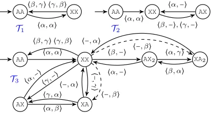
Figure 5: A graphical representation of the maximalCGfor the production cycleLR in Figure 1 and the production plant
systemS in Figure 2. A generated production controller⟨T, P⟩is as follows: T is obtained by removing indexesk from
transitions (it is thus unique); given a system historyhand an action vectora,P(h,a) =konly if a transition labelled with
a,kexists fromlast(h)(hence manyP exist). Solid and dashed lines represent controllable and uncontrollable transitions of T, respectively, andndenotes no-op−actions. For instance, by delegating the action vector⟨β,−⟩to behaviors⟨1,2⟩from
state⟨11,XX⟩(namelyβ toB1 and−toB2), the next state can either be⟨11,AX⟩or ⟨01,AX⟩, depending on the successor
state reached byB1(see Figure 2). On the other hand, the two transitions labelled with⟨−, α⟩from⟨01,AA⟩are controllable:
they represent two distinct control choices, to delegate actionαtoB2and to pauseB1or vice-versa, respectively.
or s`+1 ↝/ t`+1. In the first two cases P is not a
composi-tion. If the latter holds, it must be the case that in any trace
⟨s`+1, t`+1⟩a`+1k`+1
ÐÐÐÐÐ→⋯condition (3) of Definition 9 does not
hold, hence⟨T, P⟩is not a production controller generated
byC.
(ii)IfT′≻ T exists, then there exists a traceπsuch that
last(π)Ð→bt is in T′ for some t, but last(π)Ð→bt′ is not in T for any t′. Since T′ is realizable, there exists a
com-position P′ s.t. h ∈ Hπ,P′ whereP′(h,b) is defined, and
P(h,b)is not. So there is no trace⟨t0, s0⟩b1k1 ÐÐ→⋯b
`k`
ÐÐ→⟨t
`, s`
⟩
in C, with s0b
1k1
ÐÐ→⋯b
`k`
ÐÐ→s
`
= hand t0b
1
Ð→⋯b
`
Ð→t
`
= π, s.t. ⟨t`, s`⟩Ð→⟨b k t, s⟩for somesandk, andtas above. Then by
construction eithers`↝/ t`ors↝/ t. ◻
Computing the lazy simulation relation↝betweenS and Lmcan be done by following the algorithm for the standard
simulation relation⪰in [De Giacomoet al., 2013], but
check-ing the controllable closure tree at each step (Definition 9). An algorithm can be derived accordingly. Performance can be improved by reordering actionsaaccording to indexesk inSso as to substantially reduce the number of transitions.
6
Conclusions
In this paper we consider the parallel behavior composition problem in a manufacturing setting, where many instances of a product are to be manufactured on a production line. We introduced a novel solution concept, target production
pro-cesses, and showed how to generate the largest realizable TPP for a given production plant.
There are subtle conceptual and technical differences be-tween the parallel behavior problem and classical behavior composition in the AI literature. In particular,multiple con-current actions must be delegated to the available behaviors in the plant, rather than just one. We note that this is not the same asmultiplebehavior composition [Sardina and De Gia-como, 2008], in which several target modules are realized in the same shared available system. Multiple behavior compo-sition is equivalent to realizingLm−, which we argue is overly
demanding. Moreover, the target desired module isnotgiven as an input to the problem, but is part of the solution con-structed from the specified production recipe and plant.
Our work is just the first step in manufacturing composi-tion. We have defined the problem, and provided a notion of “adequacy” for solutions in the form of TPPs that respect re-quirementsR1-R5. Further work is needed in order torefine
m-TPPs to “efficient” manufacturing processes, for example, with respect to average throughput, machine utilization, load balancing, etc. Such optimizations can be done after the TPP has been built, or possibly during synthesis by discriminating between controllers from individual lazy simulation relations
Acknowledgments
We thank the anonymous reviewers for their helpful feedback. We acknowledge the support of the Australian Research Council (under DP120100332) and the RMIT Foundation (under an International Visiting Fellowship for the second author to visit RMIT University).
References
[Calvaneseet al., 2008] Diego Calvanese, Giuseppe De Gia-como, Maurizio Lenzerini, Massimo Mecella, and Fabio Patrizi. Automatic service composition and synthesis: The Roman Model. IEEE Data Engineering Bulletin, 31(3):18–22, 2008.
[De Giacomo and Sardina, 2007] Giuseppe De Giacomo and Sebastian Sardina. Automatic synthesis of new behaviors from a library of available behaviors. InProceedings of the International Joint Conference on Artificial Intelligence (IJCAI), pages 1866–1871, 2007.
[De Giacomoet al., 2013] Giuseppe De Giacomo, Fabio Pa-trizi, and Sebastian Sardina. Automatic behavior composi-tion synthesis.Artificial Intelligence, 196:106–142, 2013.
[Foresight, 2013] The future of manufacturing: A new era of opportunity and challenge for the UK. The Government Office for Science, London, 2013. Ref: BIS/13/810.
[Lustig and Vardi, 2009] Yoad Lustig and Moshe Y. Vardi. Synthesis from component libraries. InProceedings of the International Conference on Foundations of Software Sci-ence and Computation Structures (FoSSaCS), pages 395– 409, 2009.
[Milner, 1971] Robin Milner. An algebraic definition of sim-ulation between programs. Technical report, Stanford Uni-versity, Stanford, CA, USA, 1971.
[Sardina and De Giacomo, 2008] Sebastian Sardina and Giuseppe De Giacomo. Realizing multiple autonomous agents through scheduling of shared devices. In Pro-ceedings of the International Conference on Automated Planning and Scheduling (ICAPS), pages 304–312, 2008.
[Sardina and De Giacomo, 2009] Sebastian Sardina and Giuseppe De Giacomo. Composition of ConGolog programs. InProceedings of the International Joint Con-ference on Artificial Intelligence (IJCAI), pages 904–910, 2009.
[Stroeder and Pagnucco, 2009] Thomas Stroeder and Mau-rice Pagnucco. Realising deterministic behaviour from multiple non-deterministic behaviours. In Proceedings of the International Joint Conference on Artificial Intel-ligence (IJCAI), pages 936–941, 2009.
[Yadav and Sardina, 2012] Nitin Yadav and Sebastian Sar-dina. Qualitative approximate behavior composition. In Proceedings of the European Conference on Logics in Ar-tificial Intelligence (JELIA), volume 7519 ofLecture Notes in Computer Science (LNCS), pages 450–462. Springer, 2012.
[Yadavet al., 2013] Nitin Yadav, Paolo Felli, Giuseppe De Giacomo, and Sebastian Sardi˜na. Supremal realizability of