Difference image analysis : automatic kernel design using information criteria

Difference image analysis: automatic kernel design using information

criteria

D. M. Bramich,

Keith Horne,

K. A. Alsubai,

E. Bachelet,

D. Mislis

and N. Parley

1_{Qatar Environment and Energy Research Institute (QEERI), HBKU, Qatar Foundation, Doha, Qatar} 2_{SUPA Physics and Astronomy, North Haugh, St Andrews, Fife KY16 9SS, UK}

Accepted 2015 December 9. Received 2015 November 22; in original form 2015 August 5

A B S T R A C T

We present a selection of methods for automatically constructing an optimal kernel model for difference image analysis which require very few external parameters to control the kernel design. Each method consists of two components; namely, a kernel design algorithm to generate a set of candidate kernel models, and a model selection criterion to select the simplest kernel model from the candidate models that provides a sufficiently good fit to the target image. We restricted our attention to the case of solving for a spatially invariant convolution kernel composed of delta basis functions, and we considered 19 different kernel solution methods including six employing kernel regularization. We tested these kernel solution methods by performing a comprehensive set of image simulations and investigating how their performance in terms of model error, fit quality, and photometric accuracy depends on the properties of the reference and target images. We find that the irregular kernel design algorithm employing unregularized delta basis functions, combined with either the Akaike or Takeuchi information criterion, is the best kernel solution method in terms of photometric accuracy. Our results are validated by tests performed on two independent sets of real data. Finally, we provide some important recommendations for software implementations of difference image analysis.

Key words: methods: data analysis – methods: statistical – techniques: image processing – techniques: photometric.

1 I N T R O D U C T I O N

In astronomy, the technique of difference image analysis (DIA) aims to measure changes, from one image to another, in the objects (e.g. stars, galaxies, etc.) observed in a particular field. Typically these changes consist of variations in flux and/or position. However, the variations in the object properties that we are interested in are entangled with the differences in the sky-to-detector (or scene-to-image) transformation between pairs of images. Therefore, the DIA method must carefully model the changes in astrometry, throughput, background, and blurring between an image pair in order to extract the required astronomical information.

The state of the art in DIA has evolved substantially over the last decade and a half. Possibly the most complicated part of DIA is the optimal modelling of the convolution kernel describing the changes in point-spread function (PSF) between images. The seminal paper by Alard & Lupton (1998) set the current framework for doing this by detailing the expansion of the kernel as a linear combination of

_{E-mail:[email protected]}

basis functions. Alard (2000) subsequently showed how to model a spatially varying convolution kernel by modelling the coefficients of the kernel basis functions as polynomials of the image coordi-nates. The most important ingredient then in constructing a kernel solution in the Alard DIA framework is the definition of the set of kernel basis functions. The main developments in this area were achieved by Alard & Lupton (1998), who defined the Gaussian basis functions, Bramich (2008) and Miller, Pennypacker & White (2008) who introduced the delta basis functions (DBFs), and Becker et al. (2012, hereafterBe12) who conceived of the regularized DBFs. A detailed discussion of the kernel basis functions presented in the DIA literature may be found in Bramich et al. (2013, hereafter

Br13).

The traditional Gaussian basis functions require the specification of numerous parameters while demanding precise sub-pixel image registration for optimal results, as do many other sets of kernel basis functions (e.g. the network of bicubic B-spline functions introduced by Yuan & Akerlof 2008). Consequently, the optimal choice of parameters for generating such sets of basis functions is not obvious, although some investigation into this issue has been performed (Israel, Hessman & Schuh2007). In contrast, the DBFs have the

2016 The Authors

at University of St Andrews on March 28, 2016

http://mnras.oxfordjournals.org/

ultimate flexibility to represent a discrete kernel of any form while requiring the absolute minimal user specification; namely the kernel size and shape (or equivalently the set of ‘active’ kernel pixels). They may even be used to model fractional pixel offsets between images, avoiding the need for image resampling in the absence of other image misalignments (rotation, scale, shear, and distortion). Unsurprisingly then, DIA photometry for kernels employing DBFs has been shown to be better than that produced for kernels using Gaussian basis functions (Albrow et al.2009). However, the use of DBFs yields somewhat noisier kernel solutions than is desirable due to the relatively large number of parameters in the kernel model. To tackle this weakness of the DBFs,Be12developed the regularized DBFs through the elegant application of Tikhonov regularization to the kernel model. This refined approach produces very clean and low-noise kernel solutions at the expense of introducing an extra parameterλinto the kernel definition, where the value ofλ

controls the strength of the regularization.Be12recommend values ofλbetween 0.1 and 1 for square kernels of size 19×19 pixels although they caution that the optimal value will likely be data set dependent.

The next logical step in the development of DIA is to investigate how the properties of the image pair under consideration influence the composition of the optimal kernel model (i.e. the optimal set of DBFs, the optimal values of their coefficients, and the optimal value ofλ). In this context, ‘optimality’ refers both to the Principle of Parsimony, in that the optimal kernel model should constitute the simplest configuration of DBFs that provides a sufficiently good fit to the data, and to appropriate/relevant model performance mea-sure(s). The proposed investigation may be accomplished both by generating and analysing a comprehensive set of simulated images, and by testing on a wide variety of real image data. Neither of these tasks have yet been attempted.

Various model selection criteria have been developed from dif-ferent statistical view-points as implementations of the Principle of Parsimony (e.g. the Aikaike information criterion – Akaike1974, the Bayesian information criterion – Schwarz1978, etc.) and each one may be used to automatically select a parsimonious model from a set of models.1_{Due to the sheer number of possible combinations}

of DBFs that may constitute the kernel model, the set of models that can be considered will be limited to a set of feasible candidate kernel models defined via the adoption of an appropriate kernel de-sign algorithm. The performance of each model selection criterion may then be assessed by measuring the quality of the correspond-ing kernel solution with respect to one or more desired metric(s). The final result will then be a recommendation, dependent on the properties of the image pair under consideration, as to which model selection criterion should be adopted to consistently yield the best kernel solutions for the specified kernel design algorithm.

In this paper, we report on the results of having carried out the proposed investigation for both the unregularized and regularized DBFs (Section 2) using simulated images (Section 5) and real data (Section 6). We restrict attention to the case of solving for a spa-tially invariant convolution kernel. The performance of three pro-posed kernel design algorithms (Section 4) coupled with up to eight model selection criteria (Section 3) was assessed with regards to model error (simulations only), fit quality, and photometric accu-racy. In total, 19 methods were tested. The conclusions and recom-mendations from our investigation are detailed in Section 7.

1_{We note that the application of a model selection criterion to model fitting} may also be viewed as a regularization technique.

2 M O D E L L I N G T H E C O N VO L U T I O N K E R N E L

In this section, we briefly describe the methods used in this paper to solve for the spatially invariant convolution kernel matching the PSF between two images of the same field.

2.1 Solving for a spatially invariant kernel: recap

Consider a pair of registered images of the same field with the same dimensions and sampled on the same pixel grid. To avoid invalidating the assumption of a spatially invariant kernel model, the image registration should be such that at most there is a translational offset of a few pixels between the images, with no rotational (or other) image misalignments. Let the images be referred to as the reference imageRand the target imageIwith pixel valuesRijandIij, respectively, whereiandjare pixel indices referring to the column iand rowjof an image.

We model the target imageIas a model image Mformed by

the convolution of the reference imageRwith a spatially invariant discrete convolution kernelKplus a spatially invariant (constant2₎

differential backgroundB:

Mij =[R⊗K]ij+B, (1)

where theMijare the pixel values of the model image. As in Alard & Lupton (1998), we model Kas a linear combination of basis functions:

Krs= Nκ

q=1

aqκqrs, (2)

where theKrsare the kernel pixel values,randsare pixel indices corresponding to the columnrand rowsof the discrete kernel,Nκis

the number of kernel basis functions, and theκqrsare the pixel values of the qth discrete kernel basis function κq with corresponding coefficientaq. Substitution of equation (2) into equation (1) yields:

Mij = Nκ

q=1

aq[R⊗κq]ij+B (3)

with

[R⊗κq]ij =

rs

R(i+r)(j+s)κqrs. (4)

The image [R⊗κq]ijis referred to as abasis image. The model imageMhasNpar=Nκ+1 parameters. Note that equation (3) may

be derived as a special case of equation 8 fromBr13.

Assuming that the target-image pixel values Iij are indepen-dent observations drawn from normal (or Gaussian) distributions

N(Mij, σij) and that the parameters aqand B of the model im-age have uniform Bayesian prior probability distribution functions (PDFs), then the maximum likelihood estimator (MLE) ofaqandB may be found by minimizing the chi-squared:

χ2= ij

Iij −Mij σij

2

. (5)

This is a general linear least-squares problem (see Press et al.2007) with associatednormal equationsin matrix form:

Hα=β (6)

2_{All of the results in this paper are easily generalized to the case of a} dif-ferential background that is a polynomial function of the image coordinates (e.g. seeBr13).

at University of St Andrews on March 28, 2016

http://mnras.oxfordjournals.org/

where the symmetric and positive-definite (Nκ+ 1)×(Nκ+ 1)

matrixHis the least-squares matrix, the vectorαis the vector of Nκ+1 model parameters, andβis another vector. For the vector

of parameters:

αq=

aq for 1≤q≤Nκ

B forq=Nκ+1, (7)

the elements ofHandβare given in terms of the basis images by

Hqq= ij

ψqijψqij σ2 ij (8) βq= ij ψqijIij σ2 ij (9)

ψqij= ∂Mij

∂αq =

[R⊗κq]ij for 1≤q≤Nκ

1 forq=Nκ+1. (10)

Cholesky factorization ofH, followed by forward and back sub-stitution is the most efficient and numerically stable method (Golub & Van Loan1996) for obtaining the solutionα=αto the normal equations (i.e.αis the vector of MLEs of the model parameters). The inverse matrixH−1_{is the covariance matrix of the parameter}

es-timates cov (αq,αq )=[H−1_]

qqand consequently the uncertainty σqin eachαqis given by

σq=

[H−1_]

qq. (11)

For the spatially invariant kernel, thephotometric scale factor P between the reference and target image is a constant:

P = rs

Krs. (12)

As noted by Bramich (2008), it is good practice to subtract an estimate of the sky background level fromRbefore solving forK andBin order to minimize any correlation betweenPandB.

We adopt a noise model for the model image pixel uncertainties

σijof

σ2 ij= σ2 0 F2 ij + Mij

G Fij, (13)

whereσ0 is the CCD readout noise (ADU),Gis the CCD gain

(e−/ADU), andFij is the flat-field image. Theσijdepend on the Mijwhich renders our maximum likelihood problem as a non-linear problem and also requires that the MLE of the model image pa-rameters is obtained by minimizingχ2₊

ijln(σ

2

ij) instead ofχ2.

However, iterating the solution by considering theσijand Mij in turn as fixed is an appropriate linearization of the problem that still allows for the model image parameters to be determined by min-imizingχ2_{at each iteration as described above (since theσ}

ij are considered as constant whenever the model image parameters are being estimated). For the first iteration, we estimate theσijby ap-proximatingMijin equation (13) withIij. Ak-sigma-clip algorithm is employed at the end of each iteration except for the first to prevent outlier target-image pixel values from influencing the solution (e.g. cosmic rays, variable stars, etc.). The criterion for pixel rejection is

|εij| = |(Iij−Mij)/σij| ≥k, and we usek=4. Only 3–4 iterations are required for convergence and the final solution is highly insensitive to the initial choice ofσij(e.g. setting all of theσijto unity for the first iteration gives exactly the same result as setting theσijby ap-proximatingMijin equation 13 withIij). Finally, it should be noted

that lack of iteration introduces a bias into the kernel and differential background solution (seeBr13for a discussion and examples).

The difference imageDis defined by

Dij =Iij −Mij (14) from which we may define a normalized difference image

εij =Dij/σij. (15) In the absence of varying objects, and for a reliable noise model, the distribution of theεijvalues provides an indication of the quality of the difference image; namely, theεijshould follow a Gaussian dis-tribution with zero mean and unit standard deviation. If theεijfollow a Gaussian distribution with significant bias or standard deviation greater than unity, then systematic errors are indicated, which may be due to underfitting. If they follow a Gaussian distribution with standard deviation less than unity, then overfitting may be indicated. If they follow a non-Gaussian distribution, then an inappropriate noise model may be at least part of the cause.

2.2 The DBFs

The final ingredient required to construct a kernel solution is the definition of the set of kernel basis functions, which in turn defines the set of basis images. In this paper, we consider only theDBFs, which are defined by

κqrs=δrμδsν, (16) where a one-to-one correspondenceq↔(μ,ν) associates theqth kernel basis functionκqwith the discrete kernel pixel coordinates (μ,ν), andδijis the Kronecker delta function:

δij =

1 ifi=j

0 ifi=j . (17)

As such, each DBFκqand its corresponding coefficientaq repre-sent a single kernel pixel and its value, respectively. Note that this definition of the DBFs ignores the transformation that is required when the photometric scale factor is spatially varying (Br13).

The DBFs have a conveniently simple expression for the corre-sponding basis images:

[R⊗κq]ij =R(i+μ)(j+ν). (18)

2.3 Regularizing the DBFs

For the DBFs,Be12introduced a refinement to the normal equations to control the trade-off between noise and resolution in the kernel solution. They usedTikhonov regularization(see Press et al.2007) to penalize kernel solutions that are too noisy by adding a penalty term to the chi-squared that is derived from the second derivative of the kernel surface and whose strength is parametrized by a tuning parameterλ. The addition of a penalty term to the chi-squared is equivalent to adopting a non-uniform Bayesian prior PDF on the model parameters. The corresponding maximum penalized likeli-hood estimator (MPLE) ofaqandBis obtained by minimizing:

χ2_+λN

datαTLTLα=

ij

Iij−Mij σij

2

+λNdat

Nκ

q=1

Nκ

u=1

Nκ

v=1

aqLuqLuvav, (19)

at University of St Andrews on March 28, 2016

http://mnras.oxfordjournals.org/

whereNdatis the number of data values3(i.e. target-image pixels)

andLis an (Nκ+1)×(Nκ+1) matrix with elements: Luv = ⎧ ⎪ ⎪ ⎪ ⎪ ⎪ ⎪ ⎨ ⎪ ⎪ ⎪ ⎪ ⎪ ⎪ ⎩

Nadj,u forv=u≤Nκ, and whereNadj,uis the number of

DBFs adjacent to the DBF corresponding tou,

−1 foru≤Nκ,v≤Nκ,v=u, anduandv

corresponding to adjacent DBFs,

0 otherwise.

(20)

We consider two DBFs to beadjacent if they share a common

kernel-pixel edge,connectedif they can be linked via any number of pairs of adjacent DBFs, anddisconnectedif they are not con-nected. Note that the elements of the last row and column ofL, corresponding to the differential background parameterB, are all zero.

The matrixLis theLaplacian matrixrepresenting the connec-tivity graph of the set of DBFs (cf. graph theory). It is symmetric, diagonally dominant, and positive-semidefinite. All of the eigen-values ofLare non-negative, whileNgrp+1 of them are equal to

zero. Here,Ngrp is the number of disconnected sets of connected

DBFs within the full set of DBFs (i.e. the number of components of the connectivity graph). Consequently, the rank ofLisNκ−Ngrp,

as is the rank ofLT_{L=LL, which are facts that we will use later}

in Section 3.4. It is also useful to note that if all of the DBFs are connected to each other, thenLandLLare both of rankNκ−1.

In Appendix A, we present a couple of example kernels with their correspondingLmatrices.

The expression in equation (19) is at a minimum when its gradient with respect to each of the parametersaqandBis equal to zero. Performing the Nκ + 1 differentiations and rewriting the set of

linear equations in matrix form we obtain theregularized normal equations:

HPα=β (21)

where

HP=H+ λNdatLL. (22)

Obtaining the solution to the regularized normal equations now proceeds as for the normal equations in Section 2.1. The covariance matrix of the parameter estimatesα=αP is similarly given by

cov (αP,q,αP,q)=[H−P1]qq.

3 M O D E L S E L E C T I O N C R I T E R I A

Here, we describe our statistical tool-kit of model selection criteria that we will use for deciding on the best set of DBFs to be employed in the modelling of the convolution kernel. The criteria are valid for linear models, such as our model imageM in equation (3), and for data drawn from independent Gaussian distributions, which is a valid approximation to the Poissonian statistics of photon detection for CCD image dataIthat only breaks down at very low signal lev-els (16 e−). We direct the reader to Konishi & Kitagawa (2008) for an essential reference on the information criteria presented below.

3_{Be12accidentally omittedN}

datfrom their equation 12.

3.1 Hypothesis testing for nested models

3.1.1 χ2_-test

Theχ2_{-test may be used to compare two models A and B with}

pa-rameter setsPAandPB, respectively, that are nested (i.e.PA⊂PB).

Theχ2_{-statistic is defined by}

χ2_=χ2 A−χ

2

B, (23)

where χ2

A and χB2 are the chi-squared values of models A and

B, respectively (see equation 5). Under the null hypothesis that model B does not provide a significantly better fit than model A, theχ2_{-statistic follows a chi-squared distribution withN}

par, B−

Npar, A degrees of freedom (DoF). We set ourχ2 threshold for

rejection of the null hypothesis at 1 per cent (e.g. χ2_6.63

for DoF = 1). We adopt the chi-squared values of models A

and B as those calculated during the first iteration of our kernel solution procedure to enable a fair comparison between models since they are both computed using the same pixel uncertainties (i.e. theσij estimated by approximatingMij in equation 13 with Iij). However, the values of the model image parameters are still taken as those calculated in the final iteration of the kernel solution procedure.

Model selection using theχ2_{-test applies only to models A,}

B,..., Z with sequentially nested parameter setsPA⊂PB⊂. . . ⊂PZ.

Starting with models A and B, theχ2_{is minimized for each model}

and theχ2_{-test is used to determine whether or not model B}

pro-vides a significantly better fit than model A. If it does not, then model A is accepted as the correct model and the procedure termi-nates, otherwise the next pair of models B and C are evaluated using the same method. The procedure continues by evaluating sequential model pairs in this fashion until either theχ2_{-test indicates that}

the next model does not provide a significantly better fit or until there are no more models to test.

3.1.2 F-test

TheF-test may also be used to compare two nested models A and B. TheF-statistic is defined by

F= χ

2_/N

par,B−Npar,A

χ2 B/

Ndat−Npar,B

, (24)

where Ndat is the number of data values. Again, under the null

hypothesis that model B does not provide a significantly better fit than model A,Ffollows anF-distribution with DoF=(Npar, B−

Npar, A,Ndat−Npar, B). We set ourFthreshold for rejection of the null

hypothesis at 1 per cent (e.g.F4.63 for DoF=(2,1000)) and we compute theF-statistic using the chi-squared values of models A and B calculated during the first iteration of our kernel solution procedure. Model selection with theF-test applies to models A, B,..., Z with sequentially nested parameter sets and proceeds in the same way as model selection with theχ2_-test.

3.2 Information criteria for maximum likelihood

The principal of maximum likelihood assumes a uniform prior PDF on the model parameters. A consequence of this is that as parameters are added to a model, the maximum likelihood always increases, rendering it useless for the purpose of model selection between models with different dimensionality. Information criteria are used as an alternative for evaluating models with different numbers of

at University of St Andrews on March 28, 2016

http://mnras.oxfordjournals.org/

parameters. They may be applied regardless of whether the models under consideration are nested or non-nested.

3.2.1 AICC

The Akaike information criterion (AIC; Akaike1974) is derived as an asymptotic approximation to the Kullback–Leibler divergence (Kullback & Leibler1951),4_{which measures the distance of a}

can-didate model from the true underlying model under the assumption that the true model is of infinite dimension and is therefore not represented in the set of candidate models. The aim of the AIC is to evaluate models based on their prediction accuracy.

A version of the AIC for Gaussian linear regression problems that corrects for the small-sample bias, while being asymptotically the same as the AIC forNdatNparwas derived by Sugiura (1978):

AICC= −2 lnL(θ) +2Npar

Ndat

Ndat−Npar−1

, (25)

whereL(θ) is the likelihood function for the vector of model param-etersθ, andθis a vector of MLEs for the model parameters. Model selection with the AICCis performed by minimizing−2 lnL(θ) for

each model, and then minimizing AICCover the full set of models

under consideration.

3.2.2 TIC

The Takeuchi information criterion (TIC; Takeuchi1976) is a gen-eralization of the AIC (Konishi & Kitagawa2008) given by

TIC= −2 lnL(θ)+2tr

I(θ)J−1_(θ)

, (26)

where tr is the matrix trace operator. The matricesIandJare defined as

I(θ)= 1

Ndat

Ndat

i=1

∂lnli(θ) ∂θ

∂lnli(θ)

∂θT (27)

J(θ)= −

1

Ndat

∂2

lnL(θ)

∂θ∂θT (28)

lnL(θ)=

Ndat

i=1

lnli(θ), (29)

whereli(θ) is the likelihood function for theith (single) data point. Model selection with the TIC proceeds as for the AICC.

3.2.3 BIC

The Bayesian approach to model selection is to choose the model with the largest Bayesian posterior probability. By approximating the posterior probability of each model, Schwarz (1978) derived the Bayesian information criterion (BIC) for model selection:

BIC= −2 lnL(θ) + NparlnNdat − Nparln 2π. (30)

The BIC generally includes a heavier penalty than the AICC for

more complicated models (e.g. in the regimeNpar<20 andNdat>

4_{Use of the AIC as a model selection criterion is also equivalent to assuming} a prior PDF on the model parameters that is proportional to exp (−Npar), hence favouring models with smaller numbers of parameters.

100), therefore favouring models with fewer parameters than those favoured by the AICC. Model selection with the BIC proceeds as

for the AICC.

3.2.4 BICI

Konishi, Ando & Imoto (2004) performed a deeper Bayesian anal-ysis to derive an improved BIC:

BICI = −2 lnL(θ) +NparlnNdat

+ln(det(J(θ))) − Nparln 2π. (31)

Model selection with the BICIproceeds as for the AICC.

It is worth mentioning that the BIC and BICIareconsistentmodel

selection criteria in that they select with high probability the true model from the set of candidate models whenever the true model is represented in the set of candidate models.

3.3 Information criteria for maximum penalized likelihood

The AIC, AICC, TIC, BIC, and BICIapply only to models estimated

by maximum likelihood.

3.3.1 GICP

Konishi & Kitagawa (1996) derived a further generalization of the AIC and TIC, called the generalized information criterion (GIC), that can be applied to model selection for models with parameters estimated by maximum penalized likelihood:

GICP(λ)= −2 lnL(θP)+2tr

IP(θP)J−P1(θP)

, (32)

whereθPis a vector of MPLEs for the model parameters, and

IP(θ)=I(θ) −

λ Ndat

LT_Lθ∂lnL(θ)

∂θT (33)

JP(θ)=J(θ)+λLTL. (34)

HereLT_{Lis anN}

par×Nparmatrix and we have used the fact that

it is symmetric to slightly simplify the Konishi & Kitagawa (1996) expressions forIP(θ) andJP(θ) (their equation 21). Model selection

with the GICP(λ) is performed by minimizing GICP(λ) overλfor

each model, and then selecting the model for which GICP(λ) is

minimized over the full set of models under consideration.

3.3.2 BICP

Using the same Bayesian analysis as for the derivation of the BICI,

Konishi et al. (2004) also extended the BICIto apply to model

selec-tion for models with parameters estimated by maximum penalized likelihood. ForLT_{Lof rankN}

par−d, and denoting the product of

theNpar−dnon-zero eigenvalues ofLTLby+, they derived:

BICP(λ)= −2 lnL(θP) + dlnNdat + ln(det(JP(θP))) −dln 2π+λNdatθ

T PL

T_Lθ

P − ln+

−(Npar−d) lnλ. (35)

Model selection with the BICP(λ) proceeds as for the GICP(λ).

at University of St Andrews on March 28, 2016

http://mnras.oxfordjournals.org/

3.4 Information criteria for DIA

We may adapt the various information criteria from Sections 3.2 and 3.3 to our problem of solving for the kernel and differential back-ground in DIA. The model imageMhasNpar=Nκ+1 parameters

and we use the notationθ≡α,θ≡αandθP≡αP.

First, we compute the log-likelihood function for data drawn from Gaussian distributionsN(Mij, σij) as

−2 lnL(α)=χ2+ ij

lnσ_ij2+ Ndat ln 2π. (36)

For model selection purposes, the last termNdat ln 2πis constant

and can be ignored. Secondly, we note that since theσij are con-sidered as constant at each iteration of the maximum likelihood problem in Section 2.1, the matricesI(α) andJ(α) evaluated at α=αare given by

[I(α)]qq=

1

Ndat

ij ε2ij

ψqijψqij σ2

ij

(37)

J(α)=H/Ndat. (38)

For computational purposes it is useful to note thatI(α) is sym-metric. From these two expressions, we may derive the following results:

trI(α)J−1(α)= Ndat

Nκ+1

q=1

Nκ+1

q=1

[I(α)]qq[H−1]qq (39)

ln(det(J(α)))=ln(det(H))−(Nκ+1) lnNdat. (40)

Finally, we consider that the solution of the normal equations re-quires the computation of the Cholesky factorizationH=GGT_,

whereGis a lower triangular matrix with positive diagonal entries gqq, from which we may immediately calculate the determinant of Has det(H)=Nκ_q=+₁1g2

qq. Hence, with minimal extra computation,

the Cholesky factorization ofHyields

ln(det(H))=2

Nκ+1

q=1

lngqq. (41)

Therefore, using equations (36) and (39)–(41) for the maximum likelihood problem in Section 2.1, we have the following formulae for the relevant information criteria from Section 3.2:

AICC=χ2+

ij

lnσ_ij2+ 2(Nκ+1)

Ndat

Ndat−Nκ−2

(42)

TIC=χ2 ₊

ij

lnσ2

ij

+ 2Ndat

Nκ+1

q=1

Nκ+1

q=1

[I(α)]qq[H−1]qq

(43)

BIC=χ2 ₊

ij

lnσ2

ij

+(Nκ+1)(lnNdat − ln 2π) (44)

BICI=χ2 +

ij

lnσij2

+2

Nκ+1

q=1

lngqq − (Nκ+1) ln 2π.

(45)

Considering now the maximum penalized likelihood problem, for constantσijwe have∂lnL(α)/∂αT=βT−αTH, which is equal to λNdat(LLαP)Twhen evaluated atα=αP(using equations 21 and

22). Then, usingLT_{L=LL, the matricesI}

P(α) andJP(α) evaluated

atα=αPare given by

IP(αP)=I(αP)− λ2(L LαP)(L LαP)T (46)

JP(αP)=HP/Ndat. (47)

Writingq=Nκ

u=1

Nκ

v=1LquLuvαP,v, then, from these two

ex-pressions, we may derive the following results:

trIP(αP)J−P1(αP)

= Ndat

Nκ+1

q=1

Nκ+1

q=1

×[I(αP)]qq − λ2qq

[H−P1]qq

(48)

ln(det(JP(αP)))=ln(det(HP))−(Nκ+1) lnNdat (49)

Also, the Cholesky factorization ofHP=GPGTPyields:

ln(det(HP))=2

Nκ+1

q=1

lngP,qq. (50)

Finally, we note that the matrixLLis of rankNpar−d=Nκ−Ngrp,

and henced=Ngrp+1.

Therefore, using equations (36) and (48)–(50) for the maximum penalized likelihood problem in Section 2.3, we have the following formulae for the relevant information criteria from Section 3.3:

GICP(λ)= χ2 +

ij

lnσ2

ij

+2Ndat

Nκ+1

q=1

Nκ+1

q=1 ×[I(αP)]qq − λ2qq

[H−P1]qq (51)

BICP(λ)= χ2+

ij

lnσ2

ij

+ 2

Nκ+1

q=1

lngP,qq

−(Nκ−Ngrp) lnλNdat− (Ngrp+1) ln 2π

+λNdat

Nκ

q=1

αP,qq −ln+. (52)

4 K E R N E L D E S I G N A L G O R I T H M S

Let us introduce the concept of akernel design, which we define as a specific choice of DBFs (or, equivalently, kernel pixels) to be employed in the modelling of the convolution kernel. From a master set ofNDBFs, the model selection criteria will each select a single ‘best’ kernel design, which requires the evaluation of the criteria via the estimation of the model image parameters for each of the 2N possible kernel designs.5_{This computational problem is formidable}

and currently infeasible for values ofNthat are required for typical kernel models (e.g. a relatively small 9×9 kernel pixel grid yields

∼2.4×1024_{potential kernel designs!). Furthermore,}

branch-and-bound algorithms (e.g. Furnival & Wilson1974) for speeding up

5_{This number includes the kernel design with zero DBFs, i.e. a model image} with the differential background as the only parameter.

at University of St Andrews on March 28, 2016

http://mnras.oxfordjournals.org/

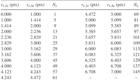
Table 1. The number of DBFs in a circular kernel design for different ranges of the kernel radiusrκ. The ranges are defined byrκ,lo≤rκ<rκ,hi. The table may be extended as appropriate for larger values ofrκ.

rκ,lo(pix) rκ,hi(pix) Nκ rκ,lo(pix) rκ,hi(pix) Nκ

0.000 1.000 1 4.472 5.000 69

1.000 1.414 5 5.000 5.099 81

1.414 2.000 9 5.099 5.385 89

2.000 2.236 13 5.385 5.657 97

2.236 2.829 21 5.657 5.831 101

2.829 3.000 25 5.831 6.000 109

3.000 3.162 29 6.000 6.083 113

3.162 3.606 37 6.083 6.325 121

3.606 4.000 45 6.325 6.403 129

4.000 4.123 49 6.403 6.708 137

4.123 4.243 57 6.708 7.000 145

4.243 4.472 61 – – –

this exhaustive search are only applicable to some of our model selection criteria in Section 3.4.

It is well known that by not considering all of the possible com-binations of predictor variables in a linear regression problem (e.g. by using stepwise regression for variable selection), the optimal set of predictors may be misidentified. However, in our case, we know from the nature/purpose of the kernel (and copious amounts of prior experience!) that the true kernel model has a peak signal at the ker-nel coordinates corresponding to the translational offset between the reference and target images (which is at the kernel origin when they are properly registered) and that this signal decays away from the peak. There may be other peaks (e.g. due to a telescope jump in the target image), but again these also have profiles that decay away from the peak(s). The best kernel designs are therefore gener-ally limited to sets of DBFs in close proximity that form relatively compact and regular shapes. Based on these observations, we have devised two algorithms for automatic kernel design that compare a manageable number of sensible kernel models; the circular ker-nel design algorithm (Section 4.1) and the irregular kerker-nel design algorithm (Section 4.2).

4.1 The circular kernel design algorithm

One very simple way to greatly reduce the number of candidate kernel designs that is in line with the expected kernel properties is to restrict the kernel designs to those that correspond to a circularly shaped pixel grid centred at the origin of the kernel pixel coordi-nates. We therefore define a circular kernel design of radiusrκas

the set of DBFs corresponding to the kernel pixels whose centres lie at or withinrκpixels of the kernel origin, which is taken to be at

the centre of the (r,s)=(0, 0) kernel pixel. Asrκis increased, the

circular kernel design includes progressively more DBFs leading to a set of nested kernel designs. In Table1, we list the number of DBFs in a circular kernel design for a range of values ofrκ.

The circular kernel design algorithm (CKDA) works for a pair of images and an adopted model selection criterion. The algorithm sequentially evaluates a set of nested model images. It finishes when the current model image under consideration fails the selection criterion, and consequently the previously considered model image is selected. For theχ2_{and F-tests, this means that the current}

model image does not provide a significantly better fit than the previous one. For the information criteria, this means that the current

model image yields a larger value of the criterion than the previous one, where λ has already been optimized individually for each model if appropriate. The algorithm proceeds as follows.

(i) Fit the model image with the differential background B as the only parameter and calculate the desired model selection criterion.

(ii) Adopt a circular kernel design of radiusrκ=0.5 pix, which

defines a kernel model with a single DBF. Fit the model image consisting of the differential background and the kernel model, and calculate the desired model selection criterion. If the model image from (i) is selected, then finish.

(iii) Incrementrκuntil the kernel model includes a new (larger)

set of DBFs. Fit the model image consisting of the differential background and the new kernel model, and calculate the desired model selection criterion. If the model image from the previous iteration is selected, then finish.

(iv) Repeat step (iii) until the algorithm terminates.

Note that the CKDA is intended to be applied to reference and target images that are registered to within a single pixel (but without requiring sub-pixel alignment necessitating image resampling).

Special care must be taken when using sigma-clipping during the fitting of the model images in the CKDA. Since each model image fit within the algorithm has the potential to clip different sets of target-image pixel values, the calculation of the model se-lection criterion may end up employing different sets of pixels at each step, which leads to undesirable jumps in its value that are unrelated to the properties of the fits. If sigma-clipping is required due to the presence of outlier pixel values, then, to avoid this prob-lem, it is recommended to run the CKDA to conclusion without using sigma-clipping and to use the selected model image to iden-tify and clip the outliers. The CKDA may then be re-run ignoring this same set of clipped pixel values at each step, and the whole process may be iterated more than once if necessary. This issue with sigma-clipping applies to all kernel design algorithms, and also whenever a fair comparison between algorithms is required (see Section 6).

In the early phases of testing the CKDA, we ran the algorithm past the finishing point to check that kernel designs with larger radii than the radius of the selected design do not yield smaller values of the information criterion, which, if this was the case, would indicate that the algorithm is terminating too early at a local minimum. We found that only in a relatively small proportion of the simulations (Section 5) a slightly smaller value of the information criterion is achieved for a kernel design with a larger radius than the selected design (usually 2–3 steps larger in Table1), and that when this occurs, the values of the model performance metrics (Section 5.2) for the two designs are very similar with no systematic improvement for the kernel design with a larger radius. Given that running the CKDA to larger radii comes at considerable cost in terms of processing power, the termination criterion of the CKDA was fixed at the first minimum of the information criterion. The same conclusions were also found to apply to the irregular kernel design algorithm (Section 4.2).

4.2 The irregular kernel design algorithm

Another way to limit the number of candidate kernel designs is to ‘grow’ the kernel model as a connected set of DBFs from a single ‘seed’ DBF by including one new DBF at each iteration. We call

at University of St Andrews on March 28, 2016

http://mnras.oxfordjournals.org/

this the irregular kernel design algorithm (IKDA), and it works for a pair of images and an adopted model selection criterion as follows.

(i) Fit the model image with the differential backgroundBas the only parameter and calculate the desired model selection criterion. (ii) Define a master set ofNDBFs by taking an appropriately large grid of kernel pixels centred on the pixel at the kernel origin. For each DBF in the master set, fit the model image consisting of the differential background and a kernel model with the single DBF, and calculate the desired model selection criterion. If the model image from (i) is selected in allNcases, then finish. Otherwise, accept the DBF from the master set that gives the best model image (according to the selection criterion) as the first DBF to be included in the kernel model (referred to as the seed DBF). Remove the seed DBF from the master set.

(iii) Find the subset of DBFs from the master set that are adjacent to at least one of the DBFs in the kernel model from the previous iteration. For each candidate DBF in this subset, fit the model image consisting of the differential background and a new kernel model with a set of DBFs that is the union of the set of DBFs in the kernel model from the previous iteration with the candidate DBF. If the model image from the previous iteration is selected in all cases, then finish. Otherwise, accept the candidate DBF that gives the best model image as the next DBF to be included in the kernel model. Remove the accepted candidate DBF from the master set.

(iv) Repeat step (iii) until the algorithm terminates.

Note that the IKDA may be applied to reference and target images that are not registered to within a single pixel since step (ii) is effectively a form of image registration. Again, special care must be taken with the application of sigma-clipping within the IKDA (see Section 4.1).

The IKDA may generate different sequences of DBFs during the growth of the kernel model for different model selection criteria. However, for theχ2_{andF-statistics, the IKDA follows the same}

sequence of DBFs since both statistics are maximized at each itera-tion of the IKDA by minimizingχ2

B. For similar reasons, the IKDA

follows the same sequence of DBFs for the AICCand the BIC. In

these cases, the different model selection criteria simply terminate the IKDA at different points in the sequence. Still, regardless of the actual model selection criterion used, we find that the IKDA always grows the kernel solution outwards from the selected seed DBF.

There are various alternative ways in which the kernel model may be grown within the IKDA. We have experimented with dropping the constraint that each new DBF must be adjacent to at least one DBF in the previous kernel model. However, this produced similar kernel solutions to those produced by the IKDA with the adjacency constraint but with an extra scattering of isolated DBFs arbitrarily far from the peak signal in the kernel. We also experimented with relaxing the definition of ‘adjacent’ to include more nearby kernel pixels, but the results from these versions of the IKDA are virtually indistinguishable in terms of the model performance metrics from the results for the IKDA described above (both for the simulated and real data). Hence we have not considered these variations on the IKDA any further.

Finally, we mention that the IKDA may be modified to generate multiple seed DBFs (possibly as part of step (ii) or by generating a new seed DBF after the algorithm terminates for the first time). This modification would be useful for adapting to situations similar to when the telescope has jumped during a target image exposure, and consequently the true kernel model consists of two or more disconnected peaks.

5 T E S T I N G AU T O M AT I C K E R N E L D E S I G N A L G O R I T H M S O N S I M U L AT E D I M AG E S

The main aim of this paper is to find out which combination of kernel design algorithm and model selection criterion consistently selects a kernel model that provides the best performance in terms of model error, fit quality, and photometric accuracy. The conclusions drawn from our investigation will likely depend on the properties of the reference and target images, and hence we must systematically map out the performance of each method accordingly. This task is most efficiently performed by generating and analysing simulated images. Furthermore, with respect to model error, the performance of each method may only be measured through the use of sim-ulations where the true model image is known. Simsim-ulations also provide a setting in which the noise model is precisely known since it is used to generate the simulated data. Thus simulations allow for the degree of under- or overfitting to be assessed accurately. For these reasons, we have performed detailed DIA simulations for a wide range of image properties.

5.1 Generating simulated images

We employed a Monte Carlo method for our investigation. We adopted reasonable values for the CCD readout noise and gain of

σ0=5 ADU andG=1 e−/ADU, respectively. For each simulation,

we generated both noiseless and noisy versions of a reference and target image pair, along with the noise maps used for generating the noisy images, via the following procedure.

(i) The size of the reference image was set to 141×141 pixels. (ii) The sky background level for the reference imageSref was

drawn from a uniform distribution on the interval [16, 1000] ADU. (iii) The log of the field star density, parametrized as the number of stars per 100 × 100 pixel image region, was drawn from a uniform distribution on the interval [0, 3], and this density was used to calculate the number of starsNstarto be generated in the reference

image.

(iv) The pixel coordinates of each star in the reference image were drawn from a uniform distribution over the image area. Also, for each star, the value ofF−3/2_{, whereFis the star flux (ADU), was}

drawn from a uniform distribution on the interval [10−9_{, 10}−9/2_].

This flux distribution is appropriate when imaging to a fixed depth through a uniform space density of stars (e.g. a good approximation for certain volumes in our Galaxy). For the purposes of performing PSF photometry on the difference image, and without loss of gen-erality, the pixel coordinates of the brightest star were modified by an integer pixel shift to lie within the central pixel of the reference image.

(v) The same normalized two-dimensional Gaussian profile of full-width at half-maximum (FWHM)fref pixels was adopted for

the profile of each star in the reference image. The value offref

was drawn from a uniform distribution on the interval [1, 6] pix, adequately covering the under- to oversampled regimes.

(vi) A square image pixel arrayRnoiselessof size 141×141 pixels

was created with all of the pixel values set to the sky background levelSref.

(vii) For each star in the reference image, the Gaussian profile was centred at the star pixel coordinates and sampled at 7 times the image resolution over the image area. The oversampled Gaussian profile was then binned (by averaging) to match the image resolution and renormalized to a sum of unity. Finally, it was scaled by the star flux and added to the imageRnoiseless.

at University of St Andrews on March 28, 2016

http://mnras.oxfordjournals.org/

(viii) An image of standard deviationsσin, ref(i.e. a noise map)

corresponding toRnoiselesswas created via

σin,ref,ij =

σ2

0+Rnoiseless,ij/G (53)

which may be derived from equation (13) by setting theFij =1.

A 141 × 141 pixel imageW of values drawn from a Gaussian

distribution with zero mean and unit standard deviation was also generated and used to construct a noisy reference imageRnoisyvia

Rnoisy,ij =Rnoiseless,ij+Wijσin,ref,ij. (54)

(ix) The size of the target image was set to 141×141 pixels. (x) For simplicity, the sky background level for the target image Starwas set toSref, which is equivalent to assuming a differential

background of zero.

(xi) A single sub-pixel shift in each of thexand yimage co-ordinate directions was drawn from a uniform distribution on the interval [−0.5, 0.5] pix and applied to the pixel coordinates of the stars in the reference image to generate the coordinates of the same stars in the target image. The fluxes of the stars in the target im-age were assumed to be the same as their fluxes in the reference image, which is equivalent to assuming non-variable stars and a photometric scale factor of unity.

(xii) The convolution kernel matching the PSF between the ref-erence and target images was assumed to be a normalized two-dimensional Gaussian profile of FWHM|fker|pixels, where a

non-negative or non-negative value offkerindicates that the kernel convolves

the reference or target image PSF, respectively. The value offker

was drawn from a uniform distribution on the interval [−1, 5] pix and the FWHMftarof the Gaussian profile for the stars in the target

image was then calculated from

f_tar2 =

f2

ref+fker2 forfker≥0

f2 ref−f

2

ker forfker<0.

(55)

(xiii) A square image pixel arrayInoiselessof size 141×141 pixels

was created with all of the pixel values set to the sky background levelStar.

(xiv) The flux profiles of the stars in the target image were added toInoiselessusing the same method as that used in step (vii) for the

reference image.

(xv) An image of standard deviations σin, tar corresponding to

Inoiselesswas created via

σin,tar,ij =

σ2

0+Inoiseless,ij/G. (56)

A new 141×141 pixel imageWof values drawn from a Gaussian distribution with zero mean and unit standard deviation was also generated and used to construct a noisy target imageInoisyvia

Inoisy,ij =Inoiseless,ij+Wijσin,tar,ij. (57)

(xvi) The imagesInoiseless,Inoisy, andσin, tarwere each trimmed to

a size of 101×101 pixels. Hence the number of data values in each simulation isNdat=10201.

(xvii) The signal-to-noise (S/N) ratio of the noisy target image SNtarwas calculated as

SNtar=

ij(Inoiseless,ij−Star)

ijσ

2 in,tar,ij

. (58)

The value of log(SNtar) is distributed approximately uniformly due

to the way the field star density is generated in step (iii). It is important to note that it does not necessarily follow that a high S/N target image has a bright high-S/N star in the centre. The high S/N

in the target image may be the consequence of the presence of a reasonable number of faint stars. In this case, the star at the centre of the image is of low S/N, even though it is the brightest star in the image.

In total, we generated the reference and target images for 548 392 simulations. We call this set of images ‘Simulation set S1’.

The above method for generating reference and target images represents the case where the reference image has approximately the same S/N ratio as the target image. However, it is common prac-tice in DIA to create a high-S/N ratio reference image by stacking images or integrating longer. We therefore also repeated the whole procedure of generating simulated images for reference images with 10 times less variance in each pixel value than the corresponding target images (or∼3.16 times better S/N). This was achieved by scaling theσin, ref,ijin step (viii) by 10−1/2∼0.316. This second set of reference and target images, ‘Simulation set S10’, was generated for a total of 529 571 simulations. Fig.1shows an example noisy reference and target image pair from one of these simulations.

5.2 Model performance metrics

We used the following metrics to measure the quality of each kernel and differential background solution.

(i) Model error. The mean squared error (MSE) measures how well the fitted model imageMmatches the true model imageInoiseless.

It is defined by

MSE= 1

Ndat

ij

(Mij−Inoiseless,ij)2. (59)

Kernel and differential background solutions with the smallest val-ues of MSE exhibit the best performance in terms of model error.

We also consider the photometric scale factorPand the differen-tial backgroundBas supplementary measures of model error. For our simulations, the closer to unity the value ofPand the closer to zero the value ofB, the better the performance of a kernel and differ-ential background solution with respect to model error. Systematic errors in the photometric scale factor are especially important since a fractional error EPinPintroduces a fractional error of EPinto the photometry (Bramich et al.2015).

(ii) Fit quality. The bias and excess variance in the fitted model image may be measured by the following statistics

MFB= 1

Ndat

ij

(Inoisy,ij−Mij) σin,tar,ij

(60)

MFV= 1

Ndat−1

ij

(Inoisy,ij−Mij) σin,tar,ij

−MFB

2

. (61)

MFB is the mean fit bias and MFV is the mean fit variance with units of sigma and sigma-squared, respectively. The closer to zero the value of MFB, and the closer to unity the value of MFV, the better the performance of a kernel and differential background solution with respect to fit quality.

(iii) Photometric accuracy. To assess the photometric accuracy, we perform PSF fitting on the difference image at the position of the brightest star in the reference image under the assumption that the reference image PSF is perfectly known. In detail, we generate a normalized two-dimensional Gaussian profile of FWHMfrefpixels

centred at the pixel coordinates of the brightest star in the reference image (guaranteed by construction to be within half a pixel of the

at University of St Andrews on March 28, 2016

http://mnras.oxfordjournals.org/

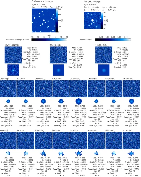
Figure 1. A reference and target image pair from simulation set S10 are shown at the top. The corresponding results for each of the 19 kernel solution methods are shown below. For each method, the difference image, kernel solution, and model performance metrics are displayed. The difference images and kernels are all displayed using the same linear scales of [−15, 15] ADU and [−0.14, 0.14], respectively. Processing times were measured for non-optimized code running on a desktop computer with an Intel Core i7-2600 CPU (3.40 GHz) and 16 Gb RAM.

at University of St Andrews on March 28, 2016

http://mnras.oxfordjournals.org/

image centre) and sampled at 7 times the image resolution. The oversampled Gaussian is then binned (by averaging) to match the image resolution, convolved with the kernel solution, trimmed in extent to a circularly shaped pixel grid of radius2ftarpixels around

the star coordinates, and renormalized. This model PSF for the target image is then optimally scaled to the difference image at the position of the brightest star by simultaneously fitting a scaling factorFdiff

and an additive constant, and using the known pixel variances in the target imageσ2

in,tar. The difference fluxFmeas of the brightest star

on the photometric scale of the reference image is then computed usingFmeas=Fdiff/P.

The theoretical minimum varianceσ2

minin the difference fluxFmeas

for PSF fitting with a scaling factor only is given by

σmin2 =

1 P2 true ⎛ ⎝ ij P2 tar,ij σ2

in,tar,ij

⎞ ⎠

−1

, (62)

wherePtrueis the true photometric scale factor (Ptrue=1 in our

sim-ulations) andPtaris the true PSF for the brightest star in the target

image (a normalized two-dimensional Gaussian profile of FWHM ftarpixels in our simulations). Since all of the stars in the

simula-tions are non-variable, the best kernel and differential background solutions should yield a distribution of values ofFmeas/σmin with

zero mean and unit variance. Hence, for a set ofNsetsimulations

indexed byk, appropriate measures for assessing the photometric accuracy are:

MPB= 1

Nset

k Fmeas,k

σmin,k

(63)

MPV= 1

Nset−1

k

Fmeas,k σmin,k

−MPB 2

. (64)

MPB is the mean photometric bias and MPV is the mean photo-metric variance with units ofσminandσmin2 , respectively. We note

that even though MPV is normalized by the theoretical minimum variance in the difference flux, it may still achieve values that are less than unity when the target image is overfit and/or when the model PSF for the target image differs from the true PSF.

5.3 Results

For each possible combination of kernel design algorithm and model selection criterion, we computed kernel and differential background solutions for all of the reference and target image pairs in both of the simulation sets S1 and S10. Furthermore, for comparison purposes, for each simulation we solved for a model image employing a square

19×19-pixel kernel design which corresponds to the unregularized kernel analysed inBe12. We also solved for the same 19×19-pixel kernel design with regularized DBFs where the optimal choice ofλ

was determined using either GICP(λ) or BICP(λ) (equations 51 and

52) which corresponds to the regularized kernel analysed inBe12. In all cases, we used three iterations for each solution, but without employing sigma-clipping since the simulated images do not suffer from outlier pixel values (see Section 2.1). The optimization ofλfor the GICPand BICPmodel selection criteria was performed using a

binary search algorithm in log (λ) for the range−3≤log (λ)≤3 with a final resolution inλof 15 per cent, while also considering the limitλ=0. Finally, the corresponding model performance metrics from Section 5.2 were calculated for each solution.

Hereafter we use a string of the form

<ALGORITHM>-<CRITERION>to refer to a specific combi-nation of kernel design algorithm (CKDA or IKDA) and model se-lection criterion (χ2_{,F, AIC}

C, TIC, GICP, BIC, BICIor BICP). For

the 19×19-pixel kernel design, we use 19×19-UNREG, 19× 19-GICP, and 19×19-BICP. Each of these combinations constitutes a

kernel solution method, and hence we have 19 methods to consider. In Fig.1, we show the difference images, kernel solutions, and model performance metrics for each of the 19 kernel solution meth-ods applied to the reference and target image pair displayed at the top (taken from simulation set S10). The target image is of medium S/N, and the reference and target images are both oversampled (withfker>2.35 pix). Notice how the regularization in the 19×

19-GICPand 19×19-BICPmethods drastically reduces the noise in the

kernel compared to the 19×19-UNREG method as demonstrated previously inBe12. Notice also how, as expected, the BIC-type cri-teria (BIC, BICI, and BICP) select kernel designs with fewer DBFs

than the kernel designs selected by the AIC-type criteria (AICC,

TIC, and GICP). Somewhat surprising is the ‘spidery’ form of the

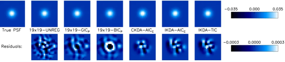
kernel solutions generated by the IKDA. A selection of model PSFs for this target image, used to perform PSF fitting on the difference images, are displayed in the top row of Fig.2alongside the true PSF for the brightest star. The residuals of these model PSFs from the true PSF (bottom row) demonstrate that the spidery form of the IKDA kernel solutions has no discernable detrimental effect, when compared to the other kernel solutions, on the convolution of the reference image PSF to obtain the target image PSF.

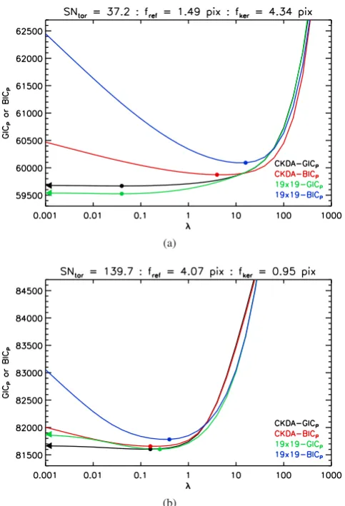
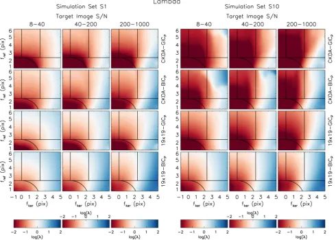
To provide an idea of what the functional forms of GICP(λ) and

BICP(λ) look like, we plot these quantities as a function ofλfor

two example simulations in Fig. 3. Each plot shows the curves for the CKDA-GICP, CKDA-BICP, 19×19-GICPand 19×19-BICP

methods. Clear minima exist indicating the optimal values ofλ. All of the simulations yield similar functional forms for GICP(λ)

and BICP(λ), and while the minima of the GICP(λ) curves may

Figure 2. The true PSF for the brightest star in the target image from Fig.1is shown at the top left. The true PSF is a normalized two-dimensional Gaussian of FWHM 4.78 pix centred in the image stamp using the sub-pixel coordinates of the brightest star. A selection of six model PSFs for the target image are shown in the top row and labelled with the corresponding kernel solution methods. The residuals of these model PSFs from the true PSF are shown in the bottom row. Each row of plots uses the linear scale reproduced at the right-hand end of the row.

at University of St Andrews on March 28, 2016

http://mnras.oxfordjournals.org/

Figure 3. Examples from the simulations of the variation of the GICPand BICPcriteria as a function ofλfor the kernel solution methods CKDA-GICP (black), CKDA-BICP(red), 19x19-GICP(green), and 19×19-BICP(blue). For the CKDA-GICPand CKDA-BICPmethods, the curves correspond to the selected kernel radius. For each curve, the minimum is marked with a filled circle. For the CKDA-GICPand 19×19-GICPmethods, the value of the curve atλ=0 is marked on the left-hand side of the plot with a triangle. Note that while GICP(λ) converges to TIC forλ→0, BICP(λ) diverges asλ→0 because of the divergence of the term involving lnλin equation (52). Hence no triangles are plotted for the CKDA-BICPand 19×19-BICP methods.

sometimes lie atλ=0, they very rarely lie at values ofλthat are greater than 10 for GICP, or that are greater than 100 for BICP.

Note that for the example shown in Fig.3(b), the optimal value of

λfor each method lies in the range 0.1–1.0 which matches with the recommendation forλfromBe12. However, for the other example shown in Fig.3(a), the GICPand BICPcriteria yield optimal values

ofλthat are<0.1 and>1.0, respectively.

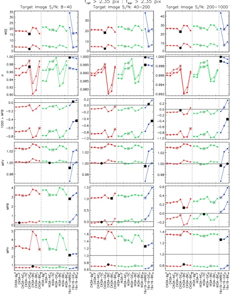
In Fig.4, for each kernel solution method we plot the median MSE,P, MFB, and MFV values, and the MPB and MPV measures, for a subset of our simulations corresponding to oversampled ref-erence images (fref ≥2.35 pix) and kernels withfker≥2.35 pix.

The corresponding plots forBare not presented because the re-sults are very similar to those forP since the photometric scale factor and differential background are correlated. We have further split the simulations into subsets based on target-image S/N (low: 8–40, medium: 40–200, high: 200–1000; three columns of plots) and reference image S/N (simulation sets S1 and S10; square or circular symbols). Similar style figures representing the results for

different subsets of simulations chosen based on image sampling are presented in Appendix B (FigsB1–B4).

Within each subset of simulations, the distributions of the vari-ous model performance metrics are single-peaked bell-shapes with rapidly falling wings and they are not far-off being Gaussian in some cases. Skewness affects some of the distributions as do a few outlier points. However, for each simulation subset and model per-formance metric, the shape and width of the distributions are very similar between the kernel solution methods. The differences in the distributions lie in their central values. Consequently, we have used the median of the model performance metrics MSE,P, MFB, and MFV in Figs4andB1–B4to compare the kernel solution methods since the median is a robust estimator of the central value. Given the Gaussian-like shape of the distributions ofFmeas/σmin, our choice

of measures MPB and MPV (equations 63 and 64) for assessing the photometric accuracy is justified.

The processing time to run the IKDA-GICP and IKDA-BICP

methods is prohibitive (see the timings noted in Fig. 1). Hence we only ran these kernel solution methods on 25 410 and 25 320 reference and target image pairs from simulation sets S1 and S10, respectively. The results from these methods are plotted in Figs4

andB1–B4, although they suffer from more noise than the other methods because they are derived from many fewer simulations. Consequently, we do not consider these two kernel solution methods any further.

5.4 Discussion

Unless otherwise stated, the discussion in this section refers to the results plotted in all of the Figs4andB1–B4, while Fig.4alone is sufficient to demonstrate the points raised.

In preparation for our discussion, it is worth considering how closely the candidate model images generated by our kernel de-sign algorithms are able represent the true underlying model image. In each simulation, the Gaussian PSF profile in the reference (or target) image is convolved with a Gaussian kernel to obtain a Gaus-sian PSF profile in the target (or reference) image. In the limits of a noiseless reference image with infinitely fine image sampling, and for a kernel that convolves the reference image, a kernel of DBFs of infinite extent is sufficient to allow for a full representation of the true underlying model image (i.e. the noiseless target image). In practice, the reference image is noisy, the reference and target im-ages are sampled at a finite scale with a spatial offset between them, the target image may be sharper than the reference image, and the kernel model employs a finite number of DBFs. It is clear therefore that none of the candidate model images will actually represent the true model image. However, for reference images with higher S/N and better sampling, and for kernel models employing more DBFs (without overfitting), the candidate model images will include mod-els that are closer to the true model. Referring back to Section 3.2, it seems then that the model selection criteria derived considering the Kullback–Leibler divergence (i.e. the AIC-type criteria) should perform the best for DIA (especially in terms of model error), and that all of the criteria should perform better with improved reference image S/N and sampling.

Unsurprisingly then, the first major conclusion that can be drawn from the results of the simulations is that with very few exceptions it is vastly advantageous, as demonstrated by all of the model per-formance metrics, to use a reference image with a higher S/N than the target image regardless of the target-image S/N, the reference or target image FWHM, or the kernel solution method employed. Our discussion will therefore focus on the results for simulation set S10.

at University of St Andrews on March 28, 2016

http://mnras.oxfordjournals.org/

Figure 4. Plots of the median MSE,P, MFB, and MFV values (equations 59, 12, 60, and 61), and the MPB and MPV measures (equations 63 and 64), for each kernel solution method forfref≥2.35 pix andfker≥2.35 pix. The results in each plot have been calculated from∼60 000 simulations for each of the simulation sets S1 and S10. Layout: the three columns of plots correspond to low (8–40), medium (40–200) and high (200–1000) S/N target images. Each row of plots corresponds to a different model performance metric. Individual plots: square and circular symbols represent the results for simulation sets S1 and S10, respectively. Red, green, and blue colours correspond to the kernel design algorithms CKDA, IKDA, and 19×19, respectively. For each algorithm, the kernel solution method with the best value of the relevant model performance metric is also plotted with an open black symbol. The method with the overall best metric value is plotted with a filled black symbol. The IKDA-GICPand IKDA-BICPmethods are excluded when determining the best metric values since their results are noisier having been determined from many fewer simulations, and because they are too computationally intensive to be of practical use with currently available computing equipment.

at University of St Andrews on March 28, 2016

http://mnras.oxfordjournals.org/