High-Resolution Self-Gated Dynamic Abdominal
MRI Using Manifold Alignment
Xin Chen
∗, Muhammad Usman, Christian F. Baumgartner, Daniel R. Balfour, Paul K. Marsden,
Andrew J. Reader, Claudia Prieto, and Andrew P. King
Abstract —We present a novel retrospective self-gating method based on manifold alignment (MA), which enables reconstruction of free breathing, high spatial, and tem-poral resolution abdominal magnetic resonance imaging sequences. Based on a radial golden-angle acquisition tra-jectory, our method enables a multidimensional self-gating signal to be extracted from thek -space data for more accu-rate motion representation. Thek -space radial profiles are evenly divided into a number of overlapping groups based on their radial angles. MA is then used to simultaneously learn and align the low dimensional manifolds of all groups, and embed them into a common manifold. In the manifold, k -space profiles that represent similar respiratory positions are close to each other. Image reconstruction is performed by combining radial profiles with evenly distributed angles that are close in the manifold. Our method was evaluated on both 2-D and 3-D synthetic andin vivo data sets. On the synthetic data sets, our method achieved high correlation with the ground truth in terms of image intensity and virtual navigator values. Using thein vivo data, compared with a state-of-the-art approach based on the center of k -space gating, our method was able to make use of much richer profile data for self-gating, resulting in statistically signifi-cantly better quantitative measurements in terms of organ sharpness and image gradient entropy.
Index Terms—Magnetic resonance imaging (MRI) reconstruction, manifold alignment (MA), MRI self-gating, respiratory motion.
I. INTRODUCTION
D
YNAMIC magnetic resonance imaging (MRI) involves imaging a region of interest with high temporal resolu-tion, and is useful in many applications in which knowledgeManuscript received November 7, 2016; accepted December 1, 2016. Date of publication January 20, 2017; date of current version April 1, 2017. This work was supported by the Engineering and Physical Sci-ences Research Council under Grant EP/M009319/1.Asterisk indicates corresponding author.
∗X. Chen is with the Division of Imaging Sciences and Biomedical
Engineering, King’s College London, London SE1 7EH, U.K. (e-mail: [email protected]).
M. Usman is with the Department of Computer Science, University College London, London WC1E 6BT, U.K.
C. F. Baumgartner is with the Biomedical Image Analysis Group, Imperial College London, London SW7 2AZ, U.K.
D. R. Balfour, P. K. Marsden, A. J. Reader, and A. P. King are with the Division of Imaging Sciences and Biomedical Engineering, King’s Col-lege London, London SE1 7EH, U.K. (e-mail: [email protected]).
C. Prieto is with the Division of Imaging Sciences and Biomedical Engineering, King’s College London, London SE1 7EH, U.K., and also with the Pontificia Universidad Catolica de Chile, Escuela de Ingenieria, Santiago, Chile.
Digital Object Identifier 10.1109/TMI.2016.2636449
of motion is of interest. For instance, dynamic MRI can help in assessing coronary artery disease [1], motion cor-rection of simultaneously acquired PET data [2], [3], or for studying the nature of respiratory motion [13]. These last two applications require a long MRI acquisition (e.g., up to 10 min in [3]) to be performed. However, the acquisition speed of MRI prevents sufficient data from being acquired quickly enough to reconstruct high-resolution fully sampled images (in both 2-D and 3-D). This problem can be tackled by using undersampled reconstruction schemes, such as com-pressed sensing (CS) [4]. CS typically involves an iterative optimization process, which can be time-consuming for large amounts of dynamic MRI data. Furthermore, motion may still occur during the period required to acquire the undersampled k-space data, especially in 3-D image acquisition. To tackle this problem, a gating approach can be used. This involves the combination of corresponding k-space data that were acquired at different times but similar motion states. Gating typically relies upon a gating signal to establish these correspondences. A range of different gating signals have been proposed, such as external-sensing-based techniques [5], [6], a pencil-beam navigator [7], and self-gating methods [8], [9]. Examples of external sensing-based methods include the use of optical tracking devices [10] or respiratory bellows [6]. Such tech-niques often involve additional setup time, may interfere with the magnetic resonance signal, or may suffer from limited field of view (FOV) or line-of-sight problems (e.g., optical tracking).
In contrast, self-gating methods address these problems by performing the gating using the acquired data themselves. A common approach is to use the magnitude of the cen-ter or central line of k-space, which is acquired continuously during the acquisition as the self-gating signal [11], [12].
Most external sensing-based methods, as well as pencil-beam navigator and current self-gating techniques, only esti-mate a simple 1-D gating signal (typically in the head foot direction). However, organ motion is a complex phenom-enon (e.g., diaphragm contraction and rib cage motion in respiratory motion), so the use of such simple signals for gating limits the quality of the reconstructed images. von Siebenthal et al. [13] developed a 4-D MRI method based on stacking of dynamic 2-D images using internal image-based sorting, which achieved better image quality than using the 1-D gating signal.
Our proposed method, which is based on manifold alignment (MA), is a self-gating method, which enables a
multidimensional signal to be used for gating. Similar to the center of k-space gating (CKG) method, the intuition behind our technique is that respiratory motion is pseudorepetitive in nature, and can, therefore, be represented by a small number of motion variables. MA is used to uncover these underlying variables. A number of previous works have reported the use of manifold learning or MA for self-gating in MRI [2], [14]–[20]. Usman et al. [20] applied Laplacian eigenmaps to estimate respiratory motion from the central intersection region of a number of consecutive k-space profiles using a radial golden-angle (RGA) acquisition [21]. Similarly, Bhatia et al. [15] used Laplacian eigenmaps to estimate cardiac motion from repetitively sampled central k-space lines using a Cartesian acquisition. Recently, Poddar and Jacob [18] used Laplacian eigenmaps to estimate both cardiac and respiratory motions from repetitively sampled radial trajectories. All of these methods were only applied in 2-D acquisition, and their extension to 3-D acquisition is not trivial as the repetitive sampling strategy reduces the scanning efficiency. In [2], we proposed a method for MRI self-gating using MA of 2-D reconstructed slices acquired at different anatomical positions. The technique worked by aligning the manifolds of manifold across slices in a groupwise fashion. Correspondences were established in the manifold and corresponding slices were stacked into volumes. In [14], the technique was extended by embedding all 2-D slices simultaneously. This was achieved by avoiding interslice data comparisons by representing each slice using a novel feature descriptor based on graph theory and random walks [22]. However, the methods in [2] and [14] are image-based self-gating methods that assumed there was no motion within each of the fully sampled 2-D image acquisitions (∼300 ms per image), which may not be true for fast motion. The use of images for self-gating also limits the achievable temporal resolution to the time taken to acquire enough data to reconstruct an entire image. To improve this technique, we have recently proposed an MA framework that is directly applied to k-space profiles [16] to achieve dynamic volume reconstruction based on a multislice 2-D acquisition. It simultaneously embeds k-space profiles that are acquired at different slices and temporal positions into a common manifold. The 3-D dynamic sequences can be reconstructed with an improved temporal resolution of∼45 ms. The above-mentioned multislice 2-D acquisition methods [2], [14], [16] assume that the underlying motions of all slices are similar, which is true for small FOV imaging (e.g., liver and heart). However, for a large FOV like the whole thorax/abdomen, it is not guaranteed that slice correspondences can be accurately established using MA.
In this paper, we adapt the MA method in [14] and propose a novel framework based on k-space MA for high spatial and temporal resolution MRI reconstruction, which is suitable for wide FOV imaging. The focus of this paper is on respiratory motion, although we believe that the technique may also be applicable to cardiac motion. Some of our prior works have been presented in [17]. We describe here the full details of the technique with some improvements, and report comprehensive evaluation results. The main novelties and contributions of this paper are summarized as follows.
1) In contrast to [15] and [20] and the CKG method, instead of using a 1-D gating signal, the proposed method performs gating in a low dimensional manifold. The use of a multidimensional gating signal and reconstruction of a high temporal resolution sequence allow better representation of the intracycle and intercycle motion variations than the CKG reconstruction of a limited number of motion states.
2) In contrast to [14], we perform MA directly on k-space data rather than the reconstructed image. This enables our technique to achieve higher temporal res-olution of the reconstructed volumes, as the fully sampled 2-D image requires ∼300 ms per image, and the acquisition of a k-space profile only takes ∼3 ms.
3) Additional to [17], we use overlapping k-space groups and an additional cost function term to achieve a more reliable MA.
4) In contrast to [2], [14], [16], our method works using a 3-D acquisition rather than a multislice 2-D acquisition, thus avoiding the assumption of a similar underlying motion across all slice positions.
5) The proposed method allows reconstruction of images at as many respiratory positions as the number k-space profiles (2-D) or the number of stacks of k-space profiles (3-D) acquired.
6) Most importantly, we demonstrate that our method works for both 2-D and 3-D acquisitions.
II. METHODOLOGY
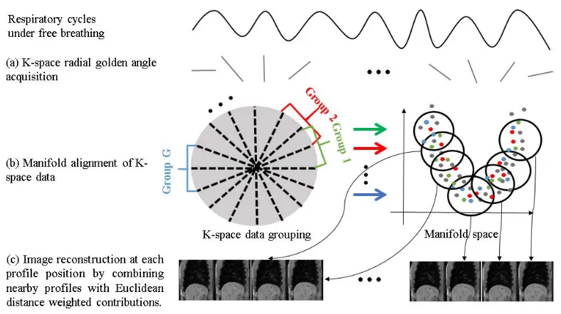
Fig. 1 provides an overview of the proposed method, which consists of k-space data acquisition, MA, and image reconstruction. During data acquisition, we acquire k-space profile data continuously under free breathing with an RGA trajectory. The temporal series of k-space lines (profiles) is then assigned to overlapping groups based only on their radial angle. Therefore, each k-space group, whilst only containing a limited range of angles in k-space, will con-tain data acquired at many different time points throughout the entire range of motion states. As such, the data in a given k-space group lie on a low dimensional manifold, which captures the range of motion states encountered during data acquisition. Rather than learning the manifold for each
k-space profile group individually, MA is used to
Fig. 1. Overview of the MA method for self-gating dynamic MRI with the following steps.(a)k-space data are acquired using RGA trajectory.
(b)Allk-space radial profiles are assigned into G overlapping groups according to their profile angles. The profiles are embedded in a low dimensional manifold using MA.(c)Image reconstruction at each profile position by combining nearby profiles with Euclidean distance weighted contributions in the manifold.
A. k-Space Data Acquisition and Grouping
Data acquisition is performed using an RGA trajectory [Fig. 1(a)] under free breathing. Compared with Cartesian acquisition, the RGA trajectory is less sensitive to motion [23], which has benefits for dynamic imaging. When acquiring profiles according to the RGA trajectory, the angle between each two consecutive profiles is 111.246°. This enables a uniform coverage of k-space with high temporal incoherence for any arbitrary number of consecutive profiles.
The k-space data are denoted by X = [x1, . . . ,xZ], where the columns xz are k-space profiles that each have S samples (k-space points in the readout direction). All radial profiles are evenly assigned to G overlapping groups according to their profile angle, where each group contains P profiles. The remaining profiles that were acquired after the K th (K =
G×P/2) are not used. As shown inFig. 1(b)(left), the black dashed lines define the angular boundaries of the groups. Each profile is a member of two adjacent overlapping groups. We only color code profiles from three (out of G) indicative groups that are correspondingly shown in the manifold in
Fig. 1(b) (right). Profiles other than those three groups are color coded as dark grey. We denote this grouped high-dimensional data as Xg, where g (1≤g≤G) is the index of
the group. Because of the RGA trajectory, the acquisition times of the radial profiles within each group are evenly distributed across the entire image acquisition period. Therefore, all of the groups share data from common respiratory cycles, and can be embedded into a common manifold with a reduced dimensionality of d. The use of overlapping groups results in a greater number of profiles for each group and, therefore, more robust alignment in the MA stage. As the central low frequency region is more important in motion estimation, we calculate a Gaussian weighting (with standard deviation
σ1) vector for each profile, centered on the central point of
the profile, denoted byv in
vs =e
−(s−S/2)2 2σ2
1 (1)
where s is the index for the k-space sample point (s=1, . . . ,S
rows of xz). We assume that the profiles within each group are comparable to each other, since they represent frequency content at approximately the same orientation (but potentially different motion states). However, because the orientations of the profiles are not exactly the same, this assumption may not be valid in high frequency regions of k-space. These Gaussian weights allow lower frequency k-space regions to contribute more than the higher frequency regions in the intragroup com-parison. Note that, for a smaller number of groups (i.e., a larger number of profiles per group, P), the central overlapping region of the profiles within the same group is smaller, and therefore, a smallerσ1is chosen. Instead of using the acquired complex data, only the magnitudes of the k-space samples weighted by v are used as the input to the subsequent MA process.
B. Manifold Alignment
minimizing a joint cost function
∅total(Y1. . .YG)= G
g=1
P
p y(pg)−
q∈η (p)
W(pqg)yq(g) 2 +μ 2 G
n=1,m=1,
m=n P
i,j
Ui j(nm)yi(n)−y(jm)2.
(2)
The first term is the locally linear embedding (LLE) cost function [24], which represents the intragroup embedding errors. LLE forms the low-dimensional manifold by preserving locally linear relations (encoded by the weight matrix W(pqg)) derived from the original high-dimensional data Xg for each group. y(pg) represents the manifold coordinates of profile p in group g. When comparing two profiles for the W(pqg) calculation, the weighted l2 norm [weights are calculated as in (1)] is used for calculating the Euclidean distance between the two profiles. Subsequently, the relations at the pth high dimensional data vector are represented by a weighted (Wpq(g)) linear combination of its KL L E nearest neighbors with index
q [q ∈η (p)].
The second term in (2) represents the intergroup cost function. yi(n) represents the manifold coordinates of profile i in group n. U(nm)is an intergroup similarity kernel, which will be discussed later. μ is a weighting parameter that balances the intragroup and intergroup terms.
The total cost function ∅total can be rewritten in matrix
form as
∅total=Tr(V H VT) (3)
where V = [Y1, . . . ,YG]is a d× (G·P) matrix containing the coordinates of the embeddings. Tr(·) is the trace operator.
H is a composition matrix that combines the intraterm and
interterm parameters, denoted as provided as shown at the bottom of this page.
The diagonal degree matrices D(nm) are given by Dii(nm)=
jU( nm)
i j . The matrices M(g) are calculated as M(g) =(I−
W(g))T(I −W(g)), where W(g) is a matrix that contains the weights(W(pqg))for the LLE term. Under the scaling constraint G
g=1YgTYg =1, the estimated embeddings V are given by the second smallest to d+1 smallest eigenvectors of H .
In our application, the groups represent k-space profiles acquired at different angles, which are not directly comparable, since they represent frequency content for different orien-tations. A key characteristic of the MA technique in [14],
which makes it suitable in our scenario, is that it performs MA without any intergroup comparisons of the original high-dimensional data. This is achieved by forming a graph in which each profile is a node. Each profile is then represented by a feature descriptor based on the steady states of random walks in the graph. This feature descriptor, denoted as f , encodes the locations of the nodes (i.e., profiles) within the graph. It enables a robust intergroup profile similarity mea-surement to be performed based on these feature descriptors via a graph matching method. Furthermore, the shared profiles of two adjacent groups (caused by the overlapping groups, see Fig. 1) enable more robust alignments of the manifolds to be made. Please refer to [14] for detailed descriptions of f . In this paper, we extend [14] to introduce an additional measurement term, which is based on the temporal positions of the two compared profiles. This allows temporally closer profiles to be embedded closer in the manifold, which results in a more reliable alignment.
The new proposed similarity measurement kernel is defined as
˜
Ui j(nm)=1−
1−e
−fi(n)−f(jm) 2
2σ2 2
1−e
−ti(n)−t(jm) 2
2σ2 3
. (4)
In (4), the first Gaussian weighted term (withσ2) is the simi-larity measurement proposed in [14], and the second Gaussian weighted term (with σ3) is the new temporal weighting mea-surement. The variable t represents the acquisition time of the corresponding profile in millisecond. As an overlapping group structure is used here, every profile is contained in two groups. For a profile that belongs to both groups n and m (i.e., when
ti(n)=t(jm)), the valueU˜i j(nm)is one, which constrains the same profile (or temporally close profiles) from the two groups to be aligned closer. As in [14], the Hungarian algorithm is used to establish one-to-one sparse correspondences between the groups of profiles by maximizing the global similarity cost. The resulting one-to-one similarity measurement Ui j(nm) from the Hungarian algorithm is used in (2). The final manifold embeddings V are solved using (3).
C. Image Reconstruction
By embedding all profiles in a common manifold, those that represent similar respiratory positions should be close together. In contrast to conventional gating methods, our method does not group the profiles into a limited number of motion states. Our method allows images to be retrospectively reconstructed at as many respiratory positions as the number of k-space
H = ⎡ ⎢ ⎢ ⎢ ⎢ ⎢ ⎢ ⎢ ⎢ ⎢ ⎣
M(1)+μ g
D(1g) −μU(12) . . . −μU(1G)
−μU(21) M(2)+μ
g
D(2g) . . . −μU(2G)
... ... ... ...
−μU(G1) −μU(G2) . . . M(G)+μ
g
D(Gg)
Fig. 2. Overview of the procedure for generating the 3-D synthetic data set. The generation of the 2-D synthetic data set follows the same procedure, with setting the slice number to be 1.
profiles (2-D) or the number of stacks of k-space profiles (3-D) acquired. For each of the acquired k-space profiles, image reconstruction is performed by grouping a number of profiles that have the closest Euclidean distances to the current profile. Duplicated profiles from two groups are only used once. To ensure that the selected profiles have an approximately even angular distribution in k-space, the L highest weighted profiles are selected from 100 evenly divided groups based on the profile radial angles, resulting in L×100 profiles being used for each of the image reconstructions. Note that the 100 groups are a fixed number, which is independent of the number of groups G. The NUFFT method [25] is used to reconstruct the final image from the selected radial k-space profiles. In contrast to the conventional NUFFT reconstruction, we use the Euclidean distances between profiles in the manifold to compute weights that determine the contributions of profiles in the nonuniform gridding process. The k-space value F(u)at each grid point u is calculated as
F(u)=
v
R(u, v)
vR(u, v)
F(v) (5)
where F(v) is the acquired k-space data value at point v from the candidate radial profiles that contribute to the data resampling at u. R(u, v) are the weighting values that are calculated from the Euclidean distances (in the manifold) of the two profiles (y(u) and y(v)) that u andv belong to
R(u, v)=c(v)×e
−y(u)−y(v)2 2σ2
4 . (6)
In (6), c(v) is the density compensation weight for the acquired k-space point v, which is calculated in the standard NUFFT process for radial trajectory. σ4 is set as half of the standard deviation of the embedded manifold coordinates. Bhatia et al. [15] used a similar manifold regression method for reconstruction but for k-space lines in a Cartesian trajec-tory. Using this weighted profile reconstruction scheme, for different profiles, different images are reconstructed even if
exactly the same sets of profiles are selected, as the weights of the profiles in each reconstruction would be different.
For 3-D image reconstruction of data acquired by the golden radial stack-of-stars method, the Fourier transform is first applied along the slice direction. This converts the z-direction encoding from the frequency domain into the image domain, where slice-by-slice reconstruction can be performed. Parameter settings for the free parameters of our method are discussed in Section III-B.
III. MATERIALS
The proposed method was evaluated on both synthetic and
in vivo data sets. The 2-D and 3-D synthetic data sets were
used to establish the ground truth to quantitatively evaluate the image reconstruction accuracy of the proposed method. We also demonstrated the practical feasibility of our technique using in vivo data sets in both 2-D and 3-D acquisitions, and the results were compared with an adapted version of the well-established CKG method.
A. 2-D and 3-D Synthetic Data Set Generation
To mimic a realistic data acquisition process, we generated high spatial and temporal resolution 3-D sequences, based on image registration of a respiratory gated high spatial resolution (RGHR) 3-D MRI volume to a dynamic 3-D low spatial resolution (DLR) MRI sequence. The DLR sequence has temporal resolution of∼260 ms and a limited number of motion states (35 in our data). Random volume selection and interpolation were used to generate a realistic ground truth sequence with high temporal resolution (∼3 ms). From this, multicoil k-space data were simulated with the same temporal resolution per k-space profile. An overview of the process is shown inFig. 2, and consists of five steps.
2) The end-exhale DLR volume was registered with all other DLR volumes [Fig. 2(b)]. Therefore, the transfor-mations were established that could deform the aligned RGHR volume to the respiratory positions of each of the DLR volumes.
3) In order to generate long and realistic synthetic dynamic sequences, the DLR volumes were grouped into four different respiratory groups (end inhale, end exhale, midinhale, and midexhale) according to their diaphragm positions in the central slice. To construct a single random respiratory cycle, we randomly selected (based on a uniform distribution) one DLR volume from each of the four groups. Using their corresponding B-spline transformations, extra DLR volumes were interpolated between these four volumes to produce a high temporal resolution breathing cycle. For the experiments in this paper, different numbers of such interpolated volumes were used to simulate slow and fast breathing cycles. For all cycles, the final synthetic sequences had a temporal resolution of∼3 ms.
4) The aligned RGHR volume was transformed to each of the respiratory states in each cycle based on the corresponding registered and interpolated B-spline trans-formations.
5) Multicoil (eight coils) images were generated for each volume using coil sensitivities simulated with an analytic integration of Biot–Savart equations. To mimic the 3-D golden angle stacof-stars acquisition [27], only one k-space profile was extracted from a single slice of each volume. The k-space profile simulation was performed along the slice direction first before moving to the next golden angle position. For the 2-D synthetic data set, the same procedure was applied with the number of slices set to 1.
The 3-D RGHR volume was acquired with respiratory gating at the end-exhale position from a volunteer, with TR= 4.4 ms, TE = 2.2 ms, flip angle =90°, acquired voxel size 2.19 ×2.19×2.74 mm3, acquired matrix size 160×160× 120, reconstructed voxel size 1.37 ×1.37 ×1.37 mm3, and reconstructed matrix size of 256×256×240. The acquisition window was approximately 100 ms, and the scan time was approximately 5 min. The 3-D DLR sequence of the same volunteer contained 35 dynamics under free breathing using cardiac gating at late diastole to minimise cardiac motion. The 3-D TFEPI was employed to acquire each volume with TR=10 ms, TE=4.9 ms, flip angle 20°, acquired voxel size 2.7 ×3.6×8.0 mm3, acquired matrix size 128×77×20, reconstructed voxel size 2.22×2.22×4.0 mm3, reconstructed matrix size 144 × 144× 40, TFE factor 26, EPI factor 13, and TFE acquisition time 267.9 ms. All the RGHR and DLR volumes were resampled into volumes with a voxel size of 1 × 1 × 1 mm3 using trilinear interpolation. In this paper, we focus on respiratory motion in the liver–lung region, and to mimic the in vivo acquisition, a region-of-interest (red box in Fig. 2) with voxel size of 1 × 1 × 8 mm3 (matrix size 200×200×10) was extracted from the original image.
To make it comparable with the in vivo acquisitions, based on the above-mentioned process, we generated 9000 multicoil
profile data for each of the 2-D data sets and 5000 multicoil stacks-of-profiles with ten sagittal slices per volume for the 3-D synthetic data sets. In total, we generated six such randomized sequences for each of the 2-D and 3-D scenarios. The data sets contained different numbers of breathing cycles ranging from 8 to 20 breathing cycles per minute. Note that, although a number of realistic motion variations are modeled by this process, some artificial motion states may be introduced due to the limitations of the registration algorithm and the interpolation process.
B. 2-D and 3-D In Vivo Data Set Acquisition
The 2-D RGA data of the liver–lung region were acquired on a Philips 1.5T scanner using a 28 channel coil on five healthy volunteers. Acquisition was performed under free breathing for approximately 30 s, resulting in approximately 9000 k-space profiles for each volunteer. A sagittal balanced SSFP acquisition was performed with 2 mm×2 mm×8 mm resolution, FOV=320 mm×320 mm, flip angle 70°, TR= 3.08 ms, and TE = 1.54 ms. The reconstructed matrix size was 160×160 with a pixel size of 2 mm× 2 mm.
For 3-D in vivo data sets, the 3-D stack-of-stars with RGA trajectory was employed for the data acquisition in the liver–lung region of five volunteers. Data were acquired on a Philips 1.5T scanner using a 28 channel coil. All profiles corresponding to one radial angle were acquired sequen-tially in the slice direction (kz) before moving to the next angle. A sagittal balanced SSFP was performed with TR =
3.8 ms, TE = 1.9 ms, FOV = 260 mm × 260 mm ×
64 mm, flip angle = 70°, resolution 2 mm × 2 mm × 8 mm, and reconstructed matrix size of 176 × 176 × 10. There were a total of 5600 stacks of profiles acquired under free breathing in approximately 5 min for each volunteer.
IV. EXPERIMENTS ANDRESULTS A. Comparative Technique
Due to the lack of ground truth for the in vivo data sets, and the fact that the conventional CKG method typically reconstructs images at a limited number of gating windows, we implemented the CKG method with adaptive gating win-dows to achieve higher temporal resolution reconstruction for comparison. For the 2-D data set, the central k-space magnitudes of all acquired radial profiles were extracted and filtered (1-D Gaussian filter with variances of 100 for 2-D data set and 10 for 3-D data set) to estimate a 1-D respiratory signal. To reconstruct a gated image at a specific profile location, a gating window (1/20 of the maximum respiratory amplitude) was set around the current profile’s
k-space magnitude. Any profiles (Kall) with a k-space mag-nitude within the gating window were assumed to represent similar respiratory positions, and the Kgatingtemporally closest profiles were selected for image reconstruction. If Kall <
to form the 1-D respiratory signal. The number of profiles used for image reconstruction was the same as for our MA-based method in order to allow a fair comparison.
B. Evaluation Criteria
1) Correlation of Virtual Navigator: Based on the syn-thetic data set, a virtual navigator (VN) [28] was used to measure the head-foot diaphragm translations of the recon-structed and the ground truth sequences. For the 2-D data set, the position of the liver–lung boundary of the sagittal view in the central column of the image was used. The central slice of the 3-D data set was used for the VN measurement by the same 2-D method. We calculated the Pearson’s correlation coefficient (PCC) between the VN values measured from the ground truth and the reconstructed sequences as one of the evaluation criteria.
2) Image Intensity Correlation: Normalized cross cor-relation (NCC) was used to compare the image intensities of the ground truth and the reconstructed sequences for the synthetic data sets. The NCC value was calculated for each corresponding pair of ground truth and reconstructed images and an overall mean and standard deviation of NCC are reported.
3) Peak Signal to Noise Ratio: The peak signal to noise ratio (PSNR) of the reconstructed synthetic data set was calculated using the corresponding ground truth sequence as the reference, as
PSNR=10log10
peakI2 MSE
(7)
where peakI is maximum value of the image’s intensity range.
MSE is the mean square error between the reconstructed image
and the ground truth image.
4) Local Sharpness:A sharpness measurement was used as a quantitative measure of image quality for both the syn-thetic and the in vivo data sets. Five lines were selected at the liver–lung boundary (three lines), main vessel in the liver (one line), and rib region (one line). The sharpness at each line was measured as the maximum of the image gradient magnitude divided by the maximum image intensity of the line [29]. The average sharpness value of the five lines was used as an eval-uation criterion for each image. The sharpness values are in the range [0, 1], and sharper structures have higher sharpness values.
5) Gradient Entropy: For both the synthetic and in
vivo data sets, the entropy was calculated based on the
gradient magnitude of the image [30]. Lower gradient entropy (GE) values indicate fewer image reconstruction artifacts.
C. Parameter Tuning
As described in Section III-A, we generated six synthetic data sets for each of the 2-D and 3-D cases. For both 2-D and 3-D, validation was performed using a two-fold cross valida-tion on the six data sets, i.e., the free parameters were tuned using one fold and applied to the other fold. The evaluation
criterion for parameter tuning was the sum of image intensity correlation (IIC) and correlation of VN (CVN).
The performance of our MA-based technique is mainly dependent on the number of profiles per group P and the number of groups G, where the product of P and G is the total number of profiles K . A larger P enables each group to contain more sampled profiles, which makes manifold embeddings more robust. On the other hand, a larger G means a smaller angular difference between the sampled profiles within each group, which enables a larger k-space region to be used for a richer comparison of profile data. Hence, a balance between P and G needs to be achieved. In order to capture the intercycle and intracycle variations, a sufficient number of samples per breathing cycle per group ( A) are essential. The number of breathing cycles (B) is automatically determined from the central k-space magnitude. G is then calculated as [K/P ×2]. The weight μ that balances the intragroup and intergroup terms in (1) is determined by the cross validation as described in the following.
Performance was found not to be sensitive to the remaining parameters, which we determined through a parameter sweep on one 2-D and one 3-D synthetic data set. The following settings were consistently applied to both 2-D and 3-D cases.
KLLE is the number of neighbors used to estimate the local relationships for the LLE, which was set as [P/10] with the minimum of 15. σ1 is the Gaussian weighting for the radial profiles, which was automatically determined by the angular range per group, calculated as [G/2π] with minimum of 3 for cases of very small G. Furthermore, σ2 (Gaussian weighting for similarity kernel) and σ3 (temporal constraint in the manifold) were set to 0.1 and 150 ms, respectively. The dimensionality of the manifold was set to 3, as suggested in [2]. Finally, L (number of selected profiles from 100 evenly distributed groups for image reconstruction) was [I×π/100], with the reconstructed image size of I×I .
For the two-fold cross validation, we varied the parameters
A and μ based on three data sets, and applied the opti-mum A and μ that achieved the best performance to the remaining three data sets. The process was then switched. The evaluation range of μ was [10−5, 10−4, 10−3, 10−2, 10−1, 100, 101] for both the 2-D and 3-D cases. The evaluation ranges of A for 2-D and 3-D tests were [10,20, . . . ,150] and [5,10,15, . . . ,30], respectively. Parameter A for 3-D data sets had a smaller range, because fewer samples were acquired per breath cycle due to the data acquisition along the slice direction.
Fig. 3. Embedded profiles in the manifold using the MA method, based on(a)2-D synthetic data set with 9000 profiles and(b)3-D synthetic data set with 5000 stacks of profiles. Eachk-space profile or stack of profiles is represented as a dot in the manifold. The profiles were color coded using the normalized centralk-space magnitude.(c)Example reconstructed images of a 3D synthetic dataset at slice positions 3, 5 and 7, using the MA method (top row). The absolute difference image between the reconstructed image using MA and the ground truth (bottom row).
TABLE I
OPTIMUMPARAMETERSETTINGS FOR2-DAND3-D SYNTHETICDATASETS
D. Evaluation Results of 2-D and 3-D Synthetic Data Sets
The two-fold cross validation results for the synthetic data sets are reported in this section. Since a multicoil acquisition was simulated, the data from only one coil that were most sensitive to the respiratory motion were automatically selected for the MA process. The coil that had the highest spectral magnitude, which was derived from the time-series k-space center values, in the frequency range of 0.5–2.5 Hz was used [25]. The profiles were then embedded into a common manifold, in which each point represents a profile. A sample embedding is shown inFig. 3(a). The colors used to visualize the embedded points were determined by the normalized magnitude of the central k-space value, and these values were used only for visualization purposes and not to determine the embeddings. As can be seen, the proposed MA method successfully embedded profiles that represent similar respira-tory positions close together. Furthermore, it has successfully captured both intracycle and intercycle variations in respiratory motion. More investigations are performed to explore this
TABLE II
EVALUATIONRESULTS FOR2-DAND3-D SYNTHETICDATASETS. THE
VALUESREPORTED IN THETABLEARE THEMEAN±STANDARD
DEVIATION OFALLSIXSYNTHETICSEQUENCES
behavior for the in vivo data set in Section IV-E. Note also that the points visualized inFig. 3(a)represent k-space profiles with a range of different angles, as the manifold is a common space for embedding all angular groups.
For the 3-D synthetic data set with 5000 stacks of profiles, it was assumed that there was no significant motion for the simulated acquisition for a given radial angle along the slice direction (i.e., for one stack of profiles). The only difference from the 2-D method was that the stack of profiles at the same radial angle was concatenated to form a single vector to be used by the MA method. The parameter settings described in Section III-C were used. An example manifold embedding is shown inFig. 3(b).
Fig. 4. (a)Virtual navigator values of the reconstructed sequence of a 2-D synthetic data set and its corresponding ground truth. Pearson’s correlation coefficient is 0.9866.(b)Virtual navigator values of the reconstructed sequence of a 3-D synthetic data set and its corresponding ground truth. Pearson’s correlation coefficient is 0.9813.
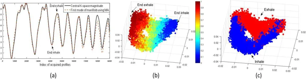
Fig. 5. (a)Magnitudes of the center ofk-space for the 2-Din vivodata set to illustrate the breathing cycles and the first mode of manifold obtained using MA.(b)Manifold embeddings of the 2-Din vivodata set with colors derived from the magnitudes of the center ofk-space. (c) Color coded embeddings that demonstrate the capability of MA to automatically distinguish between inspiration and expiration processes.
E. Evaluation Results of 2-D and 3-D In Vivo Data Sets The proposed method was also evaluated on 2-D and 3-D
in vivo data sets (Section III-A) of five healthy volunteers.
The parameter settings were the same as the first fold of the synthetic data set ( A = 80 for 2-D and A = 20 for 3-D). Also, as with the synthetic data, the profiles from the coil that was most sensitive to the respiratory motion were used for the MA process. Subsequent image reconstruction was performed using data from all coils. The normalized magnitude of the center of k-space [Fig. 5(a)] was used to color code the embedded points. In Fig. 5(a), the first mode of the manifold obtained using the MA method is also plotted for comparison, which correlates (PCC of 0.98) well with the
k-space magnitude. The 3-D manifold embedding of a sample
2-D in vivo data set is shown in Fig. 5(b). Similar to the synthetic data set, the multidimensional manifold embedding of the 2-D in vivo data set captures significant amounts of intracycle and intercycle variations. In Fig. 5(c), we show the same embedding as Fig. 5(b)but using a different color coding, which shows inspiration and expiration profiles using blue and red, respectively. It is clearly observed that the inhale and exhale profiles are automatically distinguished by the 3-D manifold embedding. This represents the well-known
hystere-sis effect, in which the motion states passed through during
inspiration are different to those passed through during expi-ration [31]. The entire dynamic sequence of the 2-D in vivo
data set was reconstructed. Since the ground truth is unknown for the in vivo data sets, the CKG method (Section IV-A) was used for comparison purposes. Fig. 6 shows example images that were reconstructed by the CKG method (top row) and our MA method (bottom row) at four different respiratory positions. Less motion and radial streaking artifacts can be observed with the proposed method, especially at small structures.
[image:9.612.57.562.244.375.2]Fig. 6. Example of 2-D reconstructed images from anin vivoacquisition at end inhale, mid exhale, end exhale, and mid inhale respiratory positions, respectively, in both full size and zoomed-in view versions. Top row and bottom row are the results using CKG and MA methods, respectively.
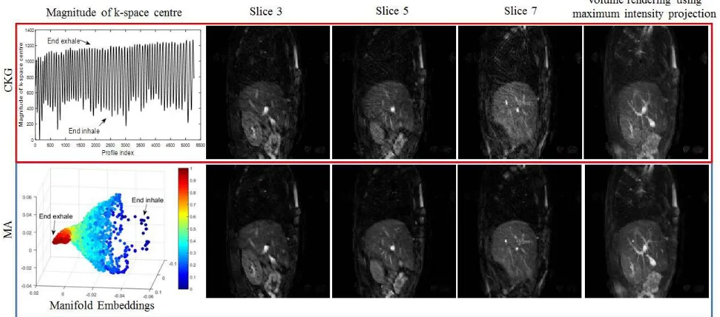
Fig. 7. Example of reconstructed 3-Din vivodata set using the CKG (top row) and the proposed MA method (bottom row). Images from left to right are reconstructed images at slice positions 3, 5, and 7, and the volume rendering result using maximum intensity projection method.
TABLE III
EVALUATIONRESULTS FOR2-DAND3-DIn VivoDATASETS. THE
VALUESREPORTED IN THETABLEARE THEMEAN±STANDARD
DEVIATIONOVERALLFIVEIn VivoDATASETS
V. CONCLUSION ANDDISCUSSION
We have presented a novel technique for retrospective dynamic MRI reconstruction, based on MA. The method enables reconstruction of “motion-free” abdominal images
throughout entire respiratory cycles. Our method was eval-uated on both 2-D and 3-D synthetic and in vivo data sets. We have shown both visually and quantitatively the improve-ment of using the MA method against the CKG method. Statis-tically, significant improvements were found in the numerical comparisons, in terms of image intensity, VN measurement, PSNR, LS, and gradient entropy (GE).
[image:10.612.53.300.612.669.2]of the entire profile rather than only the central value as in CKG. This is made possible, because our manifold embedding process only ever compares k-space data within a group, where all data are comparable and differences will be due to motion only. The use of richer profile data in the embedding process permits better estimation of underlying intracycle and intercycle variations in respiratory motion, as can be seen from the separation of inspiration and expiration profiles in
Fig. 5(b)and(c). This separation was consistently observed for all in vivo data sets. However, it is worth noting that inspiration and expiration are only separable in the manifold embeddings when large enough numbers of samples per breathing cycle are acquired (e.g., as in the 2-D acquisition). It is more difficult to capture such variations in the 3-D acquisition [Figs. 3(b) and 7], because the greater time taken to acquire a stack of profiles means that fewer such stacks are acquired in each breathing cycle.
Another key contribution of our approach is that we per-form 3-D MRI MA self-gating directly using the k-space data. To the best of our knowledge, all manifold-learning-based self-gating techniques to date have worked in 2-D only [15], [18], [20]. Those techniques would be nontrivial to extend to 3-D. Previous works in [15] and [18] involve a repetitive acquisition of certain k-space lines either in a Cartesian or radial trajectory. Therefore, significant motion is likely to occur during the additional acquisition along the slice direction in 3-D. With the RGA acquisition in [20], the intersection region of a number of consecutive spokes was used for the manifold embedding. To extend this technique to 3-D would require a multiple 2-D slice by slice acquisition, and the motion state correspondences between slices would be unknown. To address this issue, we have recently proposed a different MA framework for multislice acquisitions [16].
Our results show that impressive reconstructions can be achieved in both 2-D and 3-D. The weighted profile image reconstruction scheme efficiently uses profiles from other nearby motion states, which potentially reduces the total num-ber of profiles to be acquired, when compared with conven-tional CKG. The computaconven-tional time for MA is proporconven-tional to the total number of profiles. For 5000 stacks-of-profiles in 3-D, it takes about 60 min to run the MA on a 3.6-GHz processor with nonoptimised MATLAB code. The majority of the time are occupied by the Hungarian algorithm for establishing intergroup correspondences. The image reconstruction time is similar to a standard NUFFT reconstruction time. We modified the NUFFT code (without CS) in [25] with our weighted profile reconstruction. It takes about 50 s to reconstruct a 176×176×10 voxels 3-D volume, which is significantly less than the CS method. However, we do not view our MA method as an alternative to CS techniques, but rather a complementary approach.
As for other self-gating methods, our MA method cannot achieve a good reconstruction if an insufficient number of pro-files are available at similar respiratory positions. This would happen if, for example, an extreme inhale position was visited relatively infrequently during the imaging period. In future work, we plan to address this problem by investigating if the extreme positions could be detected by calculating the
variations of the weights that contributed to the reconstruction. Higher variation than a predefined threshold could indicate a higher likelihood of poor reconstruction quality, so this information could be used to trigger reconstruction using an alternative but more time-consuming technique like CS.
Another area for future work is to extend our method to other sampling trajectories. We believe that our MA-based framework could be applied to Cartesian sampling trajectories. In this case, groupings of k-space profiles would be based on Cartesian rows rather than radial angles. Work is also in progress to extract signals from data that are corrupted by both cardiac and respiratory motions.
In the conclusion, we believe that our proposed MA-based self-gating method for dynamic MRI represents an improve-ment on the current state of the art, and a novel application for MA in MRI imaging. The better quality and considerably higher temporal resolution reconstructed dynamic images will be useful in a range of applications, such as motion correction of PET data in a simultaneous PET-MR scenario.
DATADOWNLOAD
The data and code for generating the synthetic data sets are available at: http://kclmmag.org/downloads.html.
REFERENCES
[1] J. D. Schuijf et al., “Cardiac imaging in coronary artery disease: Differing modalities,” Heart, vol. 91, no. 8, pp. 1110–1117, 2005. [2] C. F. Baumgartner et al., “High-resolution dynamic MR imaging of
the thorax for respiratory motion correction of PET using groupwise manifold alignment,” Med. Image Anal., vol. 18, no. 7, pp. 939–952, 2014.
[3] R. Grimm et al., “Self-gated MRI motion modeling for respiratory motion compensation in integrated PET/MRI,” Med. Image Anal., vol. 19, no. 1, pp. 110–120, 2015.
[4] M. Lustig, D. Donoho, and J. M. Pauly, “Sparse MRI: The application of compressed sensing for rapid MR imaging,” Magn. Reson. Med., vol. 58, no. 6, pp. 1182–1195, 2007.
[5] A. P. King, C. Buerger, C. Tsoumpas, P. Marsden, and T. Schaeffter, “Thoracic respiratory motion estimation from MRI using a statistical model and a 2-D image navigator,” Med. Image Anal., vol. 16, no. 1, pp. 252–264, 2012.
[6] C. Santelli et al., “Respiratory bellows revisited for motion compen-sation: Preliminary experience for cardiovascular MR,” Magn. Reson.
Med., vol. 65, no. 4, pp. 1098–1103, 2011.
[7] P. G. Danias, M. V. McConnell, V. C. Khasgiwala, M. L. Chuang, R. R. Edelman, and W. J. Manning, “Prospective navigator correction of image position for coronary MR angiography,” Radiology, vol. 203, no. 3, pp. 733–736, 1997.
[8] C. Buerger, R. E. Clough, A. P. King, T. Schaeffter, and C. Prieto, “Nonrigid motion modeling of the liver from 3-D undersampled self-gated golden-radial phase encoded MRI,” IEEE Trans. Med. Imag., vol. 31, no. 3, pp. 815–905, Mar. 2012.
[9] A. C. Larson, R. D. White, G. Laub, E. R. McVeigh, D. Li, and O. P. Simonetti, “Self-gated cardiac cine MRI,” Magn. Reson. Med., vol. 51, no. 1, pp. 93–102, 2004.
[10] D. Rotenberg, M. Chiew, S. Ranieri, F. Tam, R. Chopra, and S. J. Graham, “Real-time correction by optical tracking with integrated geometric distortion correction for reducing motion artifacts in func-tional MRI,” Magn. Reson. Med., vol. 69, no. 3, pp. 734–748, 2013. [11] A. Larson, R. White, G. Laub, E. McVeigh, D. Li, and O. Simonetti,
“Self-gated cardiac cine MRI,” Magn. Reson. Imag., vol. 51, no. 1, pp. 93–102, 2004.
[13] M. V. Siebenthal, G. Székely, U. Gamper, P. Boesiger, A. Lomax, and P. Cattin, “4D MR imaging of respiratory organ motion and its variabil-ity,” Phys. Med. Biol., vol. 52, no. 6, pp. 1547–1564, 2007.
[14] C. F. Baumgartner et al., “Self-aligning manifolds for matching disparate medical image datasets,” in Proc. 24th Inf. Process. Med. Imag., 2015, pp. 363–374.
[15] K. K. Bhatia, J. Caballero, A. N. Price, Y. Sun, J. Hajnal, and D. Rueckert, “Fast reconstruction of accelerated dynamic MRI using manifold kernel regression,” in Proc. 18th Int. Conf. Med. Image
Comput. Comput. Assist. Intervent., 2015, pp. 510–518.
[16] X. Chen et al., “Dynamic volume reconstruction from multi-slice abdominal MRI using manifold alignment,” in Proc. 19th Int. Conf.
Med. Image Comput. Comput. Assist. Intervent., Athens, Greece, 2016,
pp. 493–501.
[17] X. Chen, M. Usman, C. Baumgartner, C. Prieto, and A. King, “Motion-free abdominal MRI using manifold alignment,” in Proc. Int. Soc. Magn.
Reson. Med., Singapore, 2016.
[18] S. Poddar and M. Jacob, “Dynamic MRI using smoothness regularization on manifolds (SToRM),” IEEE Trans. Med. Imag., vol. 35, no. 4, pp. 1106–1115, Apr. 2016.
[19] M. Usman, D. Atkinson, C. Kolbitsch, T. Schaeffter, and C. Prieto, “Manifold learning based ECG-free free-breathing cardiac CINE MRI,”
Magn. Reson. Imag., vol. 41, no. 6, pp. 1521–1527, 2015.
[20] M. Usman, G. Vaillant, D. Atkinson, T. Schaeffter, and C. Prieto, “Compressive manifold learning: Estimating one-dimensional respira-tory motion directly from undersampled k-space data,” Magn. Reson.
Med., vol. 72, no. 4, pp. 1130–1140, 2014.
[21] S. Winkelmann, T. Schaeffter, T. Koehler, H. Eggers, and O. Doessel, “An optimal radial profile order based on the golden ratio for time-resolved MRI,” IEEE Trans. Med. Imag., vol. 26, no. 1, pp. 68–76, Jan. 2007.
[22] M. Gori, M. Maggini, and L. Sarti, “Exact and approximate graph matching using random walks,” IEEE Trans. Pattern Anal. Mach. Intell., vol. 27, no. 7, pp. 1100–1111, Jun. 2005.
[23] G. H. Glover and J. M. Pauly, “Projection reconstruction techniques for reduction of motion effects in MRI,” Magn. Reson. Med., vol. 28, no. 2, pp. 275–289, 1992.
[24] S. T. Roweis and L. K. Saul, “Nonlinear dimensionality reduction by locally linear embedding,” Science, vol. 290, no. 5500, pp. 2323–2326, Dec. 2000.
[25] L. Feng, L. Axel, H. Chandarana, K. T. Block, D. K. Sodickson, and R. Otazo, “XD-GRASP: Golden-angle radial MRI with reconstruction of extra motion-state dimensions using compressed sensing,” Magn. Reson.
Med., vol. 75, no. 2, pp. 775–788, 2016.
[26] D. Rueckert, L. I. Sonoda, C. Hayes, D. L. G. Hill, M. O. Leach, and D. J. Hawkes, “Nonrigid registration using free-form deformations: Application to breast MR images,” IEEE Trans. Med. Imag., vol. 18, no. 8, pp. 712–721, Aug. 1999.
[27] D. C. Peters et al., “Undersampled projection reconstruction applied to MR angiography,” Magn. Reson. Med., vol. 43, no. 1, pp. 91–101, 2000.
[28] F. Savill, T. Schaeffter, and A. P. King, “Assessment of input sig-nal positioning for cardiac respiratory motion models during different breathing patterns,” in Proc. IEEE Int. Symp. Biomed. Imag., Nano
Macro, Mar./Apr. 2011, pp. 1698–1701.
[29] A. Etienne, R. M. Botnar, A. M. C. van Muiswinkel, P. Boesiger, W. J. Manning, and M. Stuber, “Soap-bubble visualization and quantitative analysis of 3D coronary magnetic resonance angiograms,” Magn. Reson. Med., vol. 48, no. 4, pp. 658–666, 2002.
[30] K. P. McGee, A. Manduca, J. P. Felmlee, S. J. Riederer, and R. L. Ehman, “Image metric-based correction (autocorrection) of motion effects: Analysis of image metrics,” J. Magn. Reson. Imag., vol. 11, no. 2, pp. 174–181, 2000.