GraphIE: A Graph Based Framework for Information Extraction

751

GraphIE: A Graph-Based Framework for Information Extraction

Yujie Qian1, Enrico Santus1, Zhijing Jin2, Jiang Guo1, and Regina Barzilay1

1_{Computer Science and Artificial Intelligence Laboratory, MIT} 2_{Department of Computer Science, The University of Hong Kong}

{yujieq, jiang guo, regina}@csail.mit.edu, {esantus, zhijing}@mit.edu

Abstract

Most modern Information Extraction (IE) sys-tems are implemented as sequential taggers and only model local dependencies. Non-local and non-sequential context is, however, a valu-able source of information to improve predic-tions. In this paper, we introduce GraphIE, a framework that operates over a graph repre-senting a broad set of dependencies between textual units (i.e. words or sentences). The al-gorithm propagates information between con-nected nodes through graph convolutions, gen-erating a richer representation that can be exploited to improve word-level predictions. Evaluation on three different tasks — namely textual, social media and visual information extraction — shows that GraphIE consistently outperforms the state-of-the-art sequence tag-ging model by a significant margin.1

1 Introduction

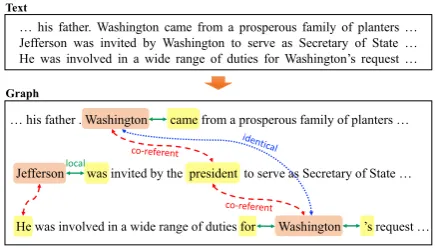
Most modern Information Extraction (IE) systems are implemented as sequential taggers. While such models effectively capture relations in the local context, they have limited capability of exploit-ing non-local and non-sequential dependencies. In many applications, however, such dependencies can greatly reduce tagging ambiguity, thereby im-proving overall extraction performance. For in-stance, when extracting entities from a document, various types of non-local contextual information such as co-references and identical mentions may provide valuable cues. See for example Figure1, in which the non-local relations are crucial to dis-criminate the entity type of the second mention of Washington(i.e. PERSONor LOCATION).

Most of the prior work looking at the non-local dependencies incorporates them by constraining

1_{Our code and data are available athttps://github.}

com/thomas0809/GraphIE.

…his father . Washington came from a prosperous family of planters…

Jefferson was invited by the president to serve as Secretary of State…

Text

Graph

He was involved in a wide range of duties for Washington ’s request … …his father. Washington came from a prosperous family of planters… Jefferson was invited by Washington to serve as Secretary of State… He was involved in a wide range of duties forWashington’srequest…

local

Figure 1: Example of the entity extraction task with an ambiguous entity mention (i.e. “...for Washing-ton’s request...”). Aside from the sentential forward and backward edges (green, solid) which aggregate lo-cal contextual information, non-lolo-cal relations — such as the co-referent edges (red, dashed) and the identical-mention edges (blue, dotted) — provide additional valuable information to reduce tagging ambiguity (i.e. PERSONor LOCATION). Best viewed in color.

the output space in a structured prediction frame-work (Finkel et al., 2005; Reichart and Barzilay, 2012; Hu et al., 2016). Such approaches, how-ever, mostly overlook the richer set of structural relations in the input space. With reference to the example in Figure 1, the co-referent depen-dencies would not be readily exploited by sim-ply constraining the output space, as they would not necessarily be labeled as entities (e.g. pro-nouns). In the attempt to capture non-local depen-dencies in the input space, alternative approaches define a graph that outlines the input structure and engineer features to describe it (Quirk and Poon, 2017). Designing effective features is however challenging, arbitrary and time consuming, espe-cially when the underlying structure is complex. Moreover, these approaches have limited capac-ity of capturing node interactions informed by the graph structure.

that improves predictions by automatically learn-ing the interactions between local and non-local dependencies in the input space. Our approach in-tegrates a graph module with the encoder-decoder architecture for sequence tagging. The algorithm operates over a graph, where nodes correspond to textual units (i.e. words or sentences) and edges describe their relations. At the core of our model, a recurrent neural network sequentially en-codes local contextual representations and then the graph module iteratively propagates information between neighboring nodes using graph convolu-tions (Kipf and Welling,2016). The learned repre-sentations are finally projected back to a recurrent decoder to support tagging at the word level.

We evaluate GraphIE on three IE tasks, namely textual, social media, and visual (Aumann et al., 2006) information extraction. For each task, we provide in input a simple task-specific graph, which defines the data structure without access to any major processing or external resources. Our model is expected to learn from the rele-vant dependencies to identify and extract the ap-propriate information. Experimental results on multiple benchmark datasets show that GraphIE consistently outperforms a strong and commonly adopted sequential model (SeqIE, i.e. a bi-directional long-short term memory (BiLSTM) followed by a conditional random fields (CRF) module). Specifically, in the textual IE task, we obtain an improvement of0.5%over SeqIE on the CONLL03 dataset, and an improvement of1.4% on the chemical entity extraction (Krallinger et al., 2015). In the social media IE task, GraphIE im-proves over SeqIE by3.7%in extracting the EDU -CATION attribute from twitter users. In visual IE, finally, we outperform the baseline by1.2%.

2 Related Work

The problem of incorporating local and non-sequential context to improve information extrac-tion has been extensively studied in the literature. The majority of methods have focused on enforc-ing constraints in the output space durenforc-ing infer-ence, through various mechanisms such as pos-terior regularization or generalized expectations (Finkel et al.,2005;Mann and McCallum,2010; Reichart and Barzilay, 2012; Li et al., 2013;Hu et al.,2016).

Research capturing non-local dependencies in the input space have mostly relied on

feature-based approaches. Roberts et al. (2008) and Swampillai and Stevenson (2011) have designed intra- and inter-sentential features based on dis-course and syntactic dependencies (e.g., short-est paths) to improve relation extraction. Quirk and Poon (2017) used document graphs to flexi-bly represent multiple types of relations between words (e.g., syntactic, adjacency and discourse re-lations).

Graph-based representations can be also learned with neural networks. The most related work to ours is the graph convolutional network by Kipf and Welling(2016), which was developed to en-code graph structures and perform node classifi-cation. In our framework, we adapt GCN as an intermediate module that learns non-local context, which — instead of being used directly for clas-sification — is projected to the decoder to enrich local information and perform sequence tagging.

A handful of other information extraction ap-proaches have used graph-based neural networks. Miwa and Bansal(2016) applied Tree LSTM (Tai et al.,2015) to jointly represent sequences and de-pendency trees for entity and relation extraction. On the same line of work, Peng et al.(2017) and Song et al.(2018) introduced Graph LSTM, which extended the traditional LSTM to graphs by en-abling a varied number of incoming edges at each memory cell. Zhang et al.(2018) exploited graph convolutions to pool information over pruned de-pendency trees, outperforming existing sequence and dependency-based neural models in a relation extraction task. These studies differ from ours in several respects. First, they can only model word-level graphs, whereas our framework can learn non-local context either from word- or sentence-level graphs, using it to reduce ambiguity during tagging at the word level. Second, all these stud-ies achieved improvements only when using de-pendency trees. We extend the graph-based ap-proach to validate the benefits of using other types of relations in a broader range of tasks, such as co-reference in named entity recognition,followed-by link in social media, and layout structure in visual information extraction.

3 Problem Definition

cap-Encoder Graph Module

Decoder

Input: Text Output: Tags

…

Encoder (BiLSTM) Decoder (BiLSTM + CRF)

Sentence 𝑖

𝐱1 (𝑖)

Sentence 𝑗

𝑣𝑖 𝑣𝑗

⋯ ⋯

…

𝑦₁(𝑖) …

𝐱2 (𝑖)

𝐱𝑘 (𝑖)

⋯

Encoder (BiLSTM) Decoder (BiLSTM + CRF)

⋯ ⋯

(a) Overview (b) Sentence-level graph

(c) Word-level graph

… 𝑦2

(𝑖)

𝑦𝑘 (𝑖)

…

𝐱1 (𝑗)

…

𝑦₁(𝑗) …

𝐱2 (𝑗)

𝐱𝑘 (𝑗)

𝑦2 (𝑗)

𝑦𝑘 (𝑗)

…

𝐱1 (𝑖)

…

𝑦1(𝑖) …

𝐱₂(𝑖) 𝐱_𝑘(𝑖) 𝑦2(𝑖) 𝑦𝑘

(𝑖)

…

…

𝐱₁(𝑗)

…

𝑦1

(𝑗) _…

𝐱2(𝑗) 𝐱𝑘 (𝑗)

𝑦2(𝑗) 𝑦𝑘 (𝑗)

Sentence 𝑖 Sentence 𝑗

⋯ ⋯

⋯ ⋯

⋯ ⋯

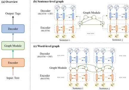
Figure 2: GraphIE framework: (a) an overview of the framework; (b) architecture forsentence-level graph, where each sentence is encoded to a node vector and fed into the graph module, and the output of the graph module is used as the initial state of the decoder; (c) architecture forword-level graph, where the hidden state for each word of the encoder is taken as the input node vector of the graph module, and then the output is fed into the decoder.

ture non-local and non-sequential dependencies between textual units, namely words or sentences. We consider the input to be a set of sentences

S = {s1, . . . , sN} and an auxiliary graph G =

(V, E), where V = {v1, . . . , vM}is the node set andE ⊂ V ×V is the edge set. Each sentence is a sequence of words. We consider two different designs of the graph:

(1) sentence-level graph, where each node is a sentence (i.e.M =N), and the edges encode sentence dependencies;

(2) word-level graph, where each node is a word (i.e. M is the number of words in the input), and the edges connect pairs of words, such as co-referent tokens.

The edgesei,j = (vi, vj) in the graph can be ei-ther directed or undirected. Multiple edge types can also be defined to capture different structural factors underlying the task-specific input data.

We use the BIO (Begin, Inside, Outside) tag-ging scheme in this paper. For each sentence

si = (w(1i), w (i) 2 , . . . , w

(i)

k ),2 we sequentially tag each word asyi = (y₁(i), y₂(i), . . . , y_k(i)).

4 Method

GraphIE jointly learns local and non-local depen-dencies by iteratively propagating information be-tween node representations. Our model has three components:

• an encoder, which generates local context-aware hidden representations for the textual unit (i.e. word or sentence, depending on the task) with a recurrent neural network;

• a graph module, which captures the graph structure, learning non-local and non-sequential dependencies between textual units;

• adecoder, which exploits the contextual in-formation generated by the graph module to perform labelling at the word level.

2_{While sentences may have different lengths, for notation}

Figure 2 illustrates the overview of GraphIE and the model architectures for both sentence- and word-level graphs. In the following sections, we first introduce the case of the sentence-level graph, and then we explain how to adapt the model for the word-level graph.

4.1 Encoder

In GraphIE, we first use an encoder to gener-ate text representations. Given a sentence si =

(w₁(i), w₂(i), . . . , w_k(i)) of lengthk, each wordw(_ti)

is represented by a vectorx(_ti), which is the con-catenation of its word embedding and a feature vector learned with a character-level convolutional neural network (CharCNN;Kim et al.(2016)). We encode the sentence with a recurrent neural net-work (RNN), defining it as

h(_1:i)_k=RNN

x(_1:i)_k;0,Θenc

, (1)

where x(_1:i)_k denotes the input sequence [x(₁i),· · ·,x_k(i)], h(_1:i)_k denotes the hidden states [h(₁i),· · · ,h(_ki)],0indicates the initial hidden state is zero, and Θenc represents the encoder

parame-ters. We implement the RNN as a bi-directional LSTM (Hochreiter and Schmidhuber, 1997), and encode each sentence independently.

We obtain the sentence representation for si by averaging the hidden states of its words, i.e. Enc(si) = 1_k

Pk

t=1h (i) t

. The sentence repre-sentations are then fed into the graph module.

4.2 Graph Module

The graph module is designed to learn the non-local and non-sequential information from the graph. We adapt the graph convolutional network (GCN) to model the graph context for information extraction.

Given the sentence-level graph G = (V, E), where each node vi (i.e. sentence si) has the encodingEnc(si) capturing its local information, the graph module enriches such representation with neighbor information derived from the graph structure.

Our graph module is a GCN which takes as input the sentence representation, i.e. g(0)_i = Enc(si), and conducts graph convolution on every node, propagating information between its neigh-bors, and integrating such information into a new hidden representation. Specifically, each layer of

GCN has two parts. The first gets the information of each node from the previous layer, i.e.

α_i(l)=W_v(l)g(_il−1), (2)

whereW(vl) is the weight to be learned. The sec-ond aggregates information from the neighbors of each node, i.e. for nodevi, we have

β(_il)= 1

d(vi)

·W(_el) X ei,j∈E

g(_jl−1)

!

, (3)

where d(vi) is the degree of node vi (i.e. the number of edges connected to vi) and is used to normalize β(_il), ensuring that nodes with dif-ferent degrees have representations of the same scale.3 _{In the simplest case, where the edges in} the graph are undirected and have the same type, we use the same weightW(el) for all of them. In a more general case, where multiple edge types exist, we expect them to have different impacts on the aggregation. Thus, we model these edge types with different weights in Eq. 3, similar to the relational GCN proposed bySchlichtkrull et al. (2018). When edges are directed, i.e. edge ei,j is different fromej,i, the propagation mechanism should mirror such difference. In this case, we consider directed edges as two types of edges (for-ward and back(for-ward), and use different weights for them.

Finally,α(_il)andβ(_il)are combined to obtain the representation at thel-th layer,

g(_il)=σα(_il)+β(_il)+b(l), (4)

where σ(·) is the non-linear activation function, andb(l)is a bias parameter.

Because each layer only propagates informa-tion between directly connected nodes, we can stack multiple graph convolutional layers to get a larger receptive field, i.e. each node can be aware of more distant neighbors. After L layers, for each node vi we obtain a contextual representa-tion,GCN(si) =g(_iL), that captures both local and non-local information.

4.3 Decoder

To support tagging, the learned representation is propagated to the decoder.

3_{We choose this simple normalization strategy instead of}

In our work, the decoder is instantiated as a BiLSTM+CRF tagger (Lample et al., 2016). The output representation of the graph module, GCN(si), is split into two vectors of the same length, which are used as the initial hidden states for the forward and backward LSTMs, respec-tively. In this way, the graph contextual infor-mation is propagated to each word through the LSTM. Specifically, we have

z(_1:i)_k =RNN

h(_1:i)_k;GCN(si),Θdec

, (5)

whereh(_1:i)_kare the output hidden states of the en-coder,GCN(si)represents the initial state, andΘdec

is the decoder parameters. A simpler way to incor-porate the graph representation into the decoder is concatenating with its input, but the empirical per-formance is worse than using as the initial state.

Finally, we use a CRF layer (Lafferty et al., 2001) on top of the BiLSTM to perform tagging,

y∗_i = arg max

y∈Yk

p

y|z(_1:i)_k; Θcrf

, (6)

whereYk is the set of all possible tag sequences of lengthk, andΘcrf represents the CRF

parame-ters, i.e. transition scores of tags. CRF combines the local predictions of BiLSTM and the transition scores to model the joint probability of the tag se-quence.4

4.4 Adaptation to Word-level Graphs

GraphIE can be easily adapted to model word-level graphs. In such case, the nodes represent words in the input, i.e. the number of nodes M

equals the total number of words in the N sen-tences. At this point, each word’s hidden state in the encoder can be used as the input node vector g_i(0) of the graph module. GCN can then con-duct graph convolution on the word-level graph and generate graph-contextualized representations for the words. Finally, the decoder directly op-erates on the GCN’s outputs, i.e. we change the BiLSTM decoder to

z(_1:i)_k=RNN

h

GCN(w(₁i)),· · ·,GCN(w_k(i))i;0,Θdec

,

4

In GraphIE, the graph module models the input space structure, i.e. the dependencies between textual units (i.e. sentences or words), and the final CRF layer models the se-quential connections of the output tags. Even though loops may exist in the input graph, CRF operates sequentially, thus the inference is tractable.

whereGCN(w(_ti))is the GCN output for wordw(_ti). In this case, the BiLSTM initial states are set to the default zero vectors. The CRF layer remains unchanged.

As it can be seen in Figure2(c), the word-level graph module differs from the sentence-level one because it directly takes the word representations from the encoder and feeds its output to the de-coder. In sentence-level graph, the GCN operates on sentence representations, which are then used as the initial states of the decoder BiLSTM.

5 Experimental Setup

We evaluate the model on three tasks, including two traditional IE tasks, namely textual informa-tion extracinforma-tion and social media informainforma-tion ex-traction, and an under-explored task —visual in-formation extraction. For each of these tasks, we created a simple task-specific graph topology, de-signed to easily capture the underlying structure of the input data without any major processing. Ta-ble1summarizes the three tasks.

5.1 Task 1: Textual Information Extraction

In this task, we focus on named entity recognition at discourse level (DiscNER). In contrast to tradi-tional sentence-level NER (SentNER), where sen-tences are processed independently, in DiscNER, long-range dependencies and constraints across sentences have a crucial role in the tagging pro-cess. For instance, multiple mentions of the same entity are expected to be tagged consistently in the same discourse. Here we propose to use this (soft) constraint to improve entity extraction.

Dataset We conduct experiments on two NER

datasets: the CoNLL-2003 dataset (CONLL03) (Tjong et al.,2003), and the CHEMDNERdataset for chemical entity extraction (Krallinger et al., 2015). We follow the standard split of each cor-pora. Statistics are shown in Table2.

Graph Construction In this task, we use a

word-level graph where nodes represent words. We create two types of edges for each document:

• Local edges: forward and backward edges are created between neighboring words in each sentence, allowing local contextual in-formation to be utilized.

Evaluation Task Graph Type Node Edge

Textual IE word-level word 1. non-local consistency (identical mentions)

2. local sentential forward and backward

Social Media IE sentence-level user’s tweets followed-by

Visual IE sentence-level text box spatial layout (horizontal and vertical)

Table 1: Comparisons of graph structure in the three IE tasks used for evaluation.

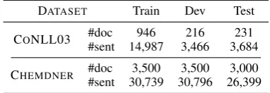
DATASET Train Dev Test

CONLL03 #doc 946 216 231

#sent 14,987 3,466 3,684

CHEMDNER #doc 3,500 3,500 3,000

#sent 30,739 30,796 26,399

Table 2: Statistics of the CONLL03 and the CHEMD-NERdatasets (Task 1).

that information can be propagated through, encouraging global consistency of tagging.5

5.2 Task 2: Social Media Information

Extraction

Social media information extraction refers to the task of extracting information from users’ posts in online social networks (Benson et al.,2011;Li et al., 2014). In this paper, we aim at extracting educationandjobinformation from users’ tweets. Given a set of tweets posted by a user, the goal is to extract mentions of the organizations to which they belong. The fact that the tweets are short, highly contextualized and show special linguistic features makes this task particularly challenging.

Dataset We construct two datasets, EDUCA

-TIONand JOB, from the Twitter corpus released by Li et al.(2014). The original corpus contains mil-lions of tweets generated by≈10thousand users, where the educationand jobmentions are anno-tated using distant supervision (Mintz et al.,2009). We sample the tweets from each user, main-taining the ratio between positive and negative posts.6The obtained EDUCATIONdataset consists of443,476tweets generated by7,208users, and the JOBdataset contains176,043tweets generated by 1,772users. Dataset statistics are reported in Table3.

5_{Note that other non-local relations such as co-references}

(cf. the example in Figure1) may be used for further im-provement. However, these relations require additional re-sources to obtain, and we leave them to future work.

6_{Positive and negative refer here to whether or not the}

ed-ucationorjobmention is present in the tweet.

EDUCATION JOB

Users 7,208 1,772

Edges 11,167 3,498

Positive Tweets 49,793 3,694

Negative Tweets 393,683 172,349

Table 3: Statistics of the EDUCATIONand JOBdatasets (Task 2).

The datasets are both split in 60% for training, 20% for development, and 20% for testing. We perform 5 different random splits and report the average results.

Graph Construction We construct the graph as

ego-networks(Leskovec and Mcauley,2012), i.e. when we extract information about one user, we consider the subgraph formed by the user and his/her direct neighbors. Each node corresponds to a Twitter user, who is represented by the set of posted tweets.7 Edges are defined by the followed-bylink, under the assumption that connected users are more likely to come from the same university or company. An example of the social media graph is reported in the appendices.

5.3 Task 3: Visual Information Extraction

Visual information extraction refers to the extrac-tion of attribute values from documents format-ted in various layouts. Examples include invoices and forms, whose format can be exploited to infer valuable information to support extraction.

Dataset The corpus consists of 25,200

Ad-verse Event Case Reports (AECR) recording drug-related side effects. Each case contains an average of 9 pages. Since these documents are produced by multiple organizations, they exhibit large vari-ability in the layout and presentation styles (e.g.

7_{As each node is a set of tweets posted by the user, we}

text, table, etc.).8 The collection is provided with a separate human-extracted ground truth database that is used as a source of distant supervision.

Our goal is to extract eight attributes related to the patient, the event, the drug and the reporter (cf. Table 6 for the full list). Attribute types include dates, words and phrases — which can be directly extracted from the document.

The dataset is split in 50% cases for training, 10% for development, and 40% for testing.

Graph Construction We first turn the PDFs

to text using PDFMiner,9 which provides words along with their positions in the page (i.e. bounding-box coordinates). Consecutive words are then geometrically joined intotext boxes. Each text box is considered as a “sentence” in this task, and corresponds to anodein the graph.

Since the page layout is the major structural fac-tor in these documents, we work on page-by-page basis, i.e. each page corresponds to a graph. The edgesare defined to horizontally or vertically con-nectnodes(text boxes) that are close to each other (i.e. when the overlap of their bounding boxes, in either the vertical or horizontal direction, is over 50%). Four types of edge are considered: left-to-right, right-to-left, up-to-down, and down-to-up. When multiple nodes are aligned, only the closest ones are connected. An example of visual docu-ment graph is reported in the appendices.

5.4 Baseline and Our Method

We implement a two-layer BiLSTM with a condi-tional random fields (CRF) tagger as the sequential baseline (SeqIE). This architecture and its variants have been extensively studied and demonstrated to be successful in previous work on information extraction (Lample et al., 2016; Ma and Hovy, 2016). In the textual IE task (Task 1), our base-line is shown to obtain competitive results with the state-of-the-art method in the CONLL03 dataset. In the visual IE task (Task 3), in order to further increase the competitiveness of the baseline, we sequentially concatenate the horizontally aligned text boxes, therefore fully modeling the horizontal edges of the graph.

Our baseline shares the same encoder and de-coder architecture with GraphIE, but without the graph module. Both architectures have similar

8

This dataset cannot be shared for patient privacy and pro-prietary issues.

9_{https://euske.github.io/pdfminer/}

DATASET Model F1

CONLL03

Lample et al.(2016) 90.94

Ma and Hovy(2016) 91.21

Ye and Ling(2018) 91.38

SeqIE 91.16

GraphIE 91.74∗

CHEMDNER

Krallinger et al.(2015) 87.39

SeqIE 88.28

GraphIE 89.71∗

Table 4: NER accuracy on the CONLL03 and the CHEMDNERdatasets (Task 1). Scores for our methods are the average of 5 runs. * indicates statistical signifi-cance of the improvement over SeqIE (p <0.01).

computational cost. In Task 1, we apply GraphIE with word-level graph module (cf. Figure 2(c)), and in Task 2 and Task 3, we apply GraphIE with sentence-level graph module (cf. Figure2(b)).

5.5 Implementation Details

The models are trained with Adam (Kingma and Ba, 2014) to minimize the CRF objective. For regularization, we choose dropout with a ratio of 0.1 on both the input word representation and the hidden layer of the decoder. The learning rate is set to 0.001. We use the development set for early-stopping and the selection of the best per-forming hyperparameters. For CharCNN, we use 64-dimensional character embeddings and 64 fil-ters of width 2 to 4 (Kim et al.,2016). The 100-dimensional pretrained GloVe word embeddings (Pennington et al., 2014) are used in Task 1 and 2, and 64-dimensional randomly initialized word embeddings are used in Task 3. We use a two-layer GCN in Task 1, and a one-two-layer GCN in Task 2 and Task 3. The encoder and decoder BiLSTMs have the same dimension as the graph convolution layer. In Task 3, we concatenate a positional en-coding to each text box’s representation by trans-forming its bounding box coordinates to a vector of length 32, and then applying atanhactivation.

6 Results

6.1 Task 1: Textual Information Extraction

Table 4 describes the NER accuracy on the CONLL03 (Tjong et al.,2003) and the CHEMD -NER(Krallinger et al.,2015) datasets.

DATASET Dictionary SeqIE GraphIE

P R F1 P R F1 P R F1

EDUCATION 78.7 93.5 85.4 85.2 93.6 89.2 92.9 92.8 92.9∗

JOB 55.7 70.2 62.1 66.2 66.7 66.2 67.1 66.1 66.5

Table 5: Extraction accuracy on the EDUCATIONand JOBdatasets (Task 2). Dictionary is a naive method which creates a dictionary of entities from the training set and extracts their mentions during testing time. Scores are the average of 5 runs. * indicates the improvement over SeqIE is statistically significant (Welch’st-test,p <0.01).

Table 1

SeqIE 94.73

random

connection 94.29 feature

augmentation 94.48 GraphIE 95.12

Dev F1

92.0 93.0 94.0 95.0 96.0

95.12 94.48

94.29 94.73

SeqIE random connection

feature augmentation

GraphIE

1

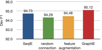
Figure 3: Analysis on the CONLL03 dataset. We com-pare with two alternative designs: (1)random connec-tion, where we replace the constructed graph by a ran-dom graph with the same number of edges; (2)feature augmentation, where we use the average embedding of each node and its neighbors as the input to the decoder, instead of the GCN which has additional parameters. We report F1 scores on the development set.

it, highlights once more the importance of mod-eling non-local and non-sequential dependencies and confirms that our approach is an appropriate method to achieve this goal.10

For CHEMDNER, we show the best performance reported inKrallinger et al.(2015), obtained with a feature-based method. Our baseline outperforms the feature-based method, and GraphIE further im-proves the performance by1.4%.

Analysis To understand the advantage of

GraphIE, we first investigate the importance of graph structure to the model. As shown in Figure3, using random connections clearly hurts the performance, bringing down the F1 score of GraphIE from 95.12% to 94.29%. It indicates that the task-specific graph structures introduce bene-ficial inductive bias. Trivial feature augmentation also does not work well, confirming the necessity of learning the graph embedding with GCN.

We further conduct error analysis on the test set to validate our motivation that GraphIE re-solves tagging ambiguity by encouraging consis-tency among identical entity mentions (cf. Figure

10_{We achieve the best reported performance among}

meth-ods not using the recently introduced ELMo (Peters et al.,

2018) and BERT (Devlin et al.,2018), which are pretrained on extra-large corpora and computationally demanding.

1). Here we examine the word-level tagging ac-curacy. We define the words that have more than one possible tags in the dataset asambiguous. We find that among the1.78%tagging errors of SeqIE, 1.16% areambiguous and 0.62%are unambigu-ous. GraphIE reduces the error rate to1.67%, with 1.06%to beambiguousand0.61%unambiguous. We can see that most of the error reduction indeed attributes to theambiguouswords.

6.2 Task 2: Social Media Information

Extraction

Table5shows the results for the social media in-formation extraction task. We first report a sim-ple dictionary-based method as a baseline. Neu-ral IE models achieve much better performance, showing that meaningful patterns are learned by the models rather than simply remembering the entities in the training set. The proposed GraphIE outperforms SeqIE in both the EDUCATION and JOBdatasets, and the improvements are more sig-nificant for the EDUCATIONdataset (3.7%versus 0.3%). The reason for such difference is the vari-ance in the affinity scores (Mislove et al., 2010) between the two datasets. Li et al. (2014) un-derline that affinity value for EDUCATIONis74.3 while for JOBit is only14.5, which means that in the datasets neighbors are5 times more likely to have studied in the same university than worked in the same company. We can therefore expect that a model like GraphIE, which exploits neighbors’ information, obtains larger advantages in a dataset characterized by higher affinity.

6.3 Task 3: Visual Information Extraction

Table6shows the results in the visual information extraction task. GraphIE outperforms the SeqIE baseline in most attributes, and achieves1.2% im-provement in the mirco average F1 score. It con-firms that the benefits of using layout graph struc-ture in visual information extraction.

ATTRIBUTE SeqIE GraphIE

P R F1 P R F1

P. Initials 93.5 92.4 92.9 93.6 91.9 92.8 P. Age 94.0 91.6 92.8 94.8 91.1 92.9 P. Birthday 96.6 96.0 96.3 96.9 94.7 95.8 Drug Name 71.2 51.2 59.4 78.5 50.4 61.4 Event 62.6 65.2 63.9 64.1 68.7 66.3 R. First Name 78.3 95.7 86.1 79.5 95.9 86.9 R. Last Name 84.5 68.4 75.6 85.6 68.2 75.9 R. City 88.9 65.4 75.4 92.1 66.3 77.1

Avg. (macro) 83.7 78.2 80.3 85.7 78.4 81.1† Avg. (micro) 78.5 73.8 76.1 80.3 74.6 77.3†

Table 6: Extraction accuracy on the AECR dataset (Task 3). Scores are the average of 5 runs. P.is the abbreviation forPatient, andR. forReporter. † indi-cates statistical significance of the improvement over SeqIE (p <0.05).

Model Dev F1

GraphIE 77.8

– Edge types 77.0 (↓0.8) – Horizontal edges 74.7 (↓3.1) – Vertical edges 72.4 (↓5.4)

– CRF 72.1 (↓5.7)

Table 7: Ablation study (Task 3). Scores are micro av-erage F1 on the development set. “–” means removing the element from GraphIE.

95.8%forPatient Birthday(similar variations are visible in the baseline). Similarly, the gap between GraphIE and SeqIE varies in relation to the at-tributes, ranging between−0.5%inPatient Birth-dayand2.4%inEvent.

In the ablation test described in Table 7, we can see the contribution of: using separate weights for different edge types (+0.8%), hor-izontal edges (+3.1%), vertical edges (+5.4%), and CRF (+5.7%).

Generalization We also assess GraphIE’s

ca-pacity of dealing with unseen layouts through an extra analysis. From our dataset, we sample2,000 reports containing the three most frequent tem-plates, and train the models on this subset. Then we test all models in two settings: 1) seen tem-plates, consisting of 1,000 additional reports in the same templates used for training; and 2) un-seen templates, consisting of1,000reports in two new template types.

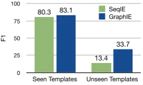
The performance of GraphIE and SeqIE is re-ported in Figure4. Both models achieve good re-sults onseen templates, with GraphIE still scoring 2.8% higher than SeqIE. The gap becomes even

Table 1

SeqIE GraphIE

Seen Templates 80.3 83.1

Unseen Templates 13.4 33.7

91.66 91.87 91.77 BiLSTM-CRF:

91.83 92.10 91.96

91.12 91.55 91.34 8%, precision: 91.78 recall: 89.39 F1: 90.57%

91.34 91.93 91.63 7%, precision: 91.90 recall: 89.14 F1: 90.50% 91.88 92.16 92.02 5%, precision: 90.88 recall: 89.62 F1: 90.25%

91.566 91.922 91.744 5%, precision: 90.49 recall: 90.24 F1: 90.37%

5%, precision: 90.53 recall: 90.25 F1: 90.39%

91.54 91.36 91.45 91.116 89.728 90.42%

91.83 91.31 91.57 90.41

90.69 90.74 90.72 91.07 90.81 90.94 91.23 91.04 91.14

91.272 91.052 91.164 GCN:

9%, precision: 91.37%, recall: 90.30%, F1: 90.83%

9%, precision: 92.03%, recall: 90.25%, F1: 91.13%

9%, precision: 92.15%, recall: 90.05%, F1: 91.09%

9%, precision: 91.23%, recall: 90.35%, F1: 90.79%

9%, precision: 92.07%, recall: 90.16%, F1: 91.10%

90.99%

90.99

F1

0 25 50 75 100

Seen Templates Unseen Templates 33.7 83.1

13.4

80.3 SeqIE

GraphIE

1

Figure 4: Micro average F1 scores tested onseenand

unseentemplates (Task 3).

larger when our model and the sequential one are tested onunseen templates (i.e. 20.3%), demon-strating that by explicitly modeling the richer structural relations, GraphIE achieves better gen-eralizability.

7 Conclusions

We introduced GraphIE, an information extraction framework that learns local and non-local con-textual representations from graph structures to improve predictions. The system operates over a task-specific graph topology describing the un-derlying structure of the input data. GraphIE jointly models the node (i.e. textual units, namely words or sentences) representations and their de-pendencies. Graph convolutions project informa-tion through neighboring nodes to finally support the decoder during tagging at the word level.

We evaluated our framework on three IE tasks, namely textual, social media and visual infor-mation extraction. Results show that it effi-ciently models non-local and non-sequential con-text, consistently enhancing accuracy and out-performing the competitive SeqIE baseline (i.e. BiLSTM+CRF).

Future work includes the exploration of auto-matically learning the underlying graphical struc-ture of the input data.

Acknowledgments

References

Yonatan Aumann, Ronen Feldman, Yair Liberzon, Benjamin Rosenfeld, and Jonathan Schler. 2006. Visual information extraction. Knowl. Inf. Syst., 10(1):1–15.

Edward Benson, Aria Haghighi, and Regina Barzilay. 2011. Event discovery in social media feeds. In

Proceedings of ACL, pages 389–398. ACL.

Jacob Devlin, Ming-Wei Chang, Kenton Lee, and Kristina Toutanova. 2018. Bert: Pre-training of deep bidirectional transformers for language understand-ing. arXiv preprint arXiv:1810.04805.

Jenny Rose Finkel, Trond Grenager, and Christopher Manning. 2005. Incorporating non-local informa-tion into informainforma-tion extracinforma-tion systems by gibbs sampling. InProceedings of ACL, pages 363–370. ACL.

Sepp Hochreiter and J¨urgen Schmidhuber. 1997. Long short-term memory. Neural computation, 9(8):1735–1780.

Zhiting Hu, Xuezhe Ma, Zhengzhong Liu, Eduard Hovy, and Eric Xing. 2016. Harnessing deep neural networks with logic rules. InProceedings of ACL, pages 2410–2420.

Yoon Kim, Yacine Jernite, David Sontag, and Alexan-der M Rush. 2016. Character-aware neural language models. InProceedings of AAAI, pages 2741–2749. AAAI Press.

Diederik P Kingma and Jimmy Ba. 2014. Adam: A method for stochastic optimization. arXiv preprint arXiv:1412.6980.

Thomas N Kipf and Max Welling. 2016. Semi-supervised classification with graph convolutional networks. arXiv preprint arXiv:1609.02907.

Martin Krallinger, Florian Leitner, Obdulia Rabal, Miguel Vazquez, Julen Oyarzabal, and Alfonso Va-lencia. 2015. Chemdner: The drugs and chemical names extraction challenge. Journal of cheminfor-matics, 7(1):S1.

John D Lafferty, Andrew McCallum, and Fernando CN Pereira. 2001. Conditional random fields: Prob-abilistic models for segmenting and labeling se-quence data. In Proceedings of ICML, pages 282– 289.

Guillaume Lample, Miguel Ballesteros, Sandeep Sub-ramanian, Kazuya Kawakami, and Chris Dyer. 2016. Neural architectures for named entity recognition. InProceedings of NAACL-HLT, pages 260–270, San Diego, California. ACL.

Jure Leskovec and Julian J Mcauley. 2012. Learning to discover social circles in ego networks. InNIPS, pages 539–547.

Jiwei Li, Alan Ritter, and Eduard Hovy. 2014. Weakly supervised user profile extraction from twitter. In

Proceedings of ACL, volume 1, pages 165–174.

Qi Li, Heng Ji, and Liang Huang. 2013. Joint event extraction via structured prediction with global fea-tures. InProceedings of ACL, volume 1, pages 73– 82.

Xuezhe Ma and Eduard Hovy. 2016. End-to-end se-quence labeling via bi-directional lstm-cnns-crf. In

Proceedings of ACL, pages 1064–1074, Berlin, Ger-many. ACL.

Gideon S Mann and Andrew McCallum. 2010. Gener-alized expectation criteria for semi-supervised learn-ing with weakly labeled data. Journal of Machine Learning Research, 11(Feb):955–984.

Mike Mintz, Steven Bills, Rion Snow, and Dan Juraf-sky. 2009. Distant supervision for relation extrac-tion without labeled data. In Proceedings of ACL, pages 1003–1011. ACL.

Alan Mislove, Bimal Viswanath, Krishna P Gummadi, and Peter Druschel. 2010. You are who you know: inferring user profiles in online social networks. In

Proceedings of the 3rd ACM International Confer-ence on Web Search and Data Mining, pages 251– 260. ACM.

Makoto Miwa and Mohit Bansal. 2016. End-to-end re-lation extraction using lstms on sequences and tree structures.arXiv preprint arXiv:1601.00770.

Nanyun Peng, Hoifung Poon, Chris Quirk, Kristina Toutanova, and Wen-tau Yih. 2017. Cross-sentence n-ary relation extraction with graph lstms. TACL, 5:101–115.

Jeffrey Pennington, Richard Socher, and Christopher Manning. 2014. Glove: Global vectors for word representation. In Proceedings of EMNLP, pages 1532–1543.

Matthew Peters, Mark Neumann, Mohit Iyyer, Matt Gardner, Christopher Clark, Kenton Lee, and Luke Zettlemoyer. 2018. Deep contextualized word rep-resentations. In Proceedings of NAACL-HLT, vol-ume 1, pages 2227–2237.

Chris Quirk and Hoifung Poon. 2017. Distant super-vision for relation extraction beyond the sentence boundary. InProceedings of ACL, volume 1, pages 1171–1182.

Roi Reichart and Regina Barzilay. 2012. Multi event extraction guided by global constraints. In Proceed-ings of NAACL-HLT, pages 70–79. ACL.

Michael Schlichtkrull, Thomas N Kipf, Peter Bloem, Rianne van den Berg, Ivan Titov, and Max Welling. 2018. Modeling relational data with graph convolu-tional networks. InEuropean Semantic Web Confer-ence, pages 593–607. Springer.

Linfeng Song, Yue Zhang, Zhiguo Wang, and Daniel Gildea. 2018. N-ary relation extraction using graph-state lstm. InProceedings of EMNLP, pages 2226– 2235.

Kumutha Swampillai and Mark Stevenson. 2011. Ex-tracting relations within and across sentences. In

Proceedings of the International Conference Recent Advances in Natural Language Processing, pages 25–32.

Kai Sheng Tai, Richard Socher, and Christopher D Manning. 2015. Improved semantic representations from tree-structured long short-term memory net-works. arXiv preprint arXiv:1503.00075.

Kim Sang Tjong, F Erik, and Fien De Meulder. 2003. Introduction to the conll-2003 shared task: Language-independent named entity recognition. In

Proceedings of NAACL-HLT, pages 142–147. ACL.

Zhixiu Ye and Zhen-Hua Ling. 2018. Hybrid semi-markov crf for neural sequence labeling. In Pro-ceedings of ACL, pages 235–240.

Yuhao Zhang, Peng Qi, and Christopher D Manning. 2018. Graph convolution over pruned dependency trees improves relation extraction. InProceedings of EMNLP.

A Appendices

We show some examples of the constructed graphs for different information extraction tasks.

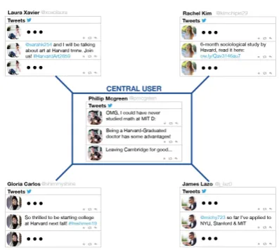
A.1 Social Media Information Extraction

Figure 5: Mock-up example of Social Media Informa-tion ExtracInforma-tion (Task 2). Nodes are represented as users and edges arefollow-byrelations.

A.2 Visual Information Extraction