Online Full Text



Abstract—In this paper, we present a distance

transform-based geometric path planning algorithm suitable for robots with vision capability. We show that the proposed approach can reduce the computation time needed to find an optimal collision-free path compared to other path planning algorithms by utilizing the output of the computer vision module and by eliminating any extra work to model the workspace of the robot. We illustrate the application of this algorithm in 2D and 3D and present two optimization algorithms to reduce the number of waypoints and shorten the Euclidean distance of the path. Finally, we show how this algorithm can be incorporated in systems with on-board sensors and how the output of the vision module can be streamed to the algorithm to allow real-time path planning.

Index Terms—path planning, collision avoidance, computer vision.

I. INTRODUCTION

Geometric path planning is a robust alternative algorithm for computing a collision free path connecting the initial and final configurations of a robot with a minimal number of waypoints in 2D and 3D environments. It provides a geometric description of the robot motion given a mapping and a description of the obstacles in the workspace. The algorithm outputs the (x,y,z) coordinates of the path in the workspace which is then passed to a custom inverse kinematics block to compute the revolute and prismatic joint variables in the configuration space. In this paper, we illustrate the application of this algorithm by computing an optimal path for the end-effector; however, this algorithm can be applied to all the origins of the Denavit Hartenburg frames or a set of floating control points in the links to ensure that the entire kinematic chain follows a collision free path. The motivation for this path planning approach is to minimize the computation time needed to find a collision free path for sensor-equipped robots by eliminating the representational cost incurred by modeling the workspace. This is done by designing the path planning algorithm around the output of the vision module, mainly the segmented image of the workspace.

II. PRIOR WORK

Most of the work on the motion planning for robots has

Manuscript received July 5, 2009.

Ziyad Aljarboua is with Harvard University, Cambridge, MA 02138 USA (phone: 617-955-1063; fax: 815-717-9838; e-mail: [email protected]).

approached the problem with the assumption that the environment in which the robot operates is completely or partially known. Based on the approach of this paper, path planning algorithms can be classified according to the extensiveness and the cost of the workspace representation. Methods like vertex graph and cell decomposition are examples of algorithms with low representational cost [1][2]. They, however, are too local and their modeling cost grows with the area of the workspace rather than the number of obstacles. The other category consists of methods that involve large overhead for the construction of the workspace model such as the quadtree and octree representations [3][4]. In these methods, the free space is hierarchically decomposed into smaller units and the findpath problem is essentially converted into a graph search problem. Algorithms like Dijkstra or A* are used in such algorithms to search the graph [5][6]. The computation cost of these methods takes (n2) time where n is the number of vertices of the obstacles [7]. Randomized potential field is a sampling-based planning method based on performing best-first search on a high or multi resolution grid and a random walk to skip local minima [8]. This method exploits best-first heuristics to solve the findpath problem without searching all grid points. It, however, involves many heuristic parameters that need to be adjusted for each problem. Path planning has also been proposed in the configuration space. Randomized preprocessing schemes used for query processing in holonomic robots configuration space path planning through the use of random sampling in the preprocessing stage [9][10]. In such methods, a probabilistic roadmap is constructed and used in the query phase. The roadmap represents a graph where the nodes correspond to collision-free configurations and the edges correspond to the paths between these configurations. These methods suffer from extended learning time in environments with complicated geometry and are limited to static workspaces.

III. THE 2D ALGORITHM

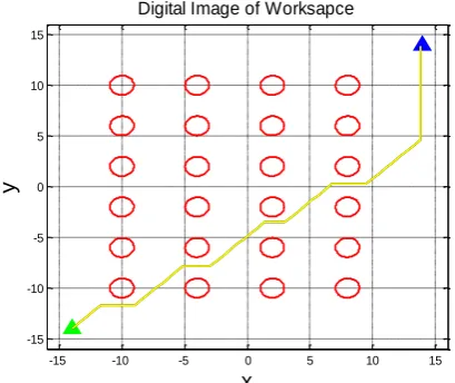
The 2D geometric path planning algorithm in which the world 𝒲= 2 is based on distance transform where the workspace is modeled as a digital image (or a distance map) with a set of occupiable positions (cells or pixels). Each cell can either be free, occupied by an obstacle or occupied by a point on the path of the robot. Figure 1 shows an example of a 60×60 distance map in 2D with cylindrical obstacles uniformly distributed throughout the workspace and an optimal path connecting the initial and final configurations. Each cell is initialized to zero to indicate a free cell and then

Geometric Path Planning for General Robot

Manipulators

the obstacle region φ ⊆𝒲 is systematically constructed by performing a one-time simple sequential scan of the workspace to assign a non-zero value to all cells occupied by obstacles. The free space then becomes . In 2D, the value of the occupied cell has no significance and it is only used to indicate the presence of an obstacle at that location. Figure 2 shows the 3D model of the workspace of figure 1 with arbitrary values assigned to the cells occupied by the obstacles. Given the initial and final position of the end-effector, and , the path is computed by recursively reevaluating the distance to the final goal from each of the neighboring cells to select the next intermediate cell that lies on the path as illustrated in figure 3. K-neighborhood for the grid, the number of cells to evaluate at each time step to determine the search depth, is set to the 8 adjacent cells. The selection of the K-neighborhood represents a tradeoff between the computation time and the length of the path. Increasing the k-neighborhood value enables the path to skip intermediate cells. This effect is offseted by the two optimization steps included in this algorithm. At each iteration, the Euclidean distance from all the 8 adjacent cells to the final position is initialized to infinity and then reassigned the actual distance if the cell is not occupied by an obstacle and it is not already part of the path. Finally, the cell with the shortest distance from the goal is selected and added to the path. This process is repeated until the distance from the goal is less than the specified tolerance ε.

IV. PATH BACKTRACKING

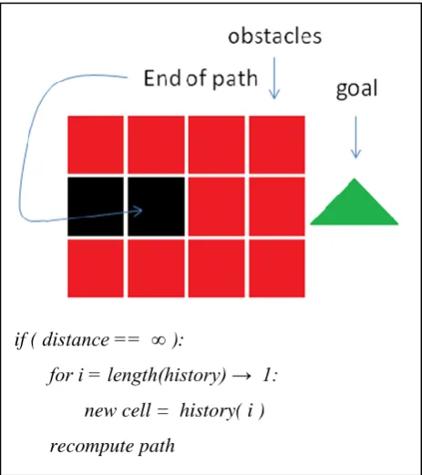
Similar to the local minima trap in the gradient descent, this algorithm can get trapped between a set of obstacles as shown in figure 4. Generally, the algorithm does not allow any cell that lies on the path to be occupied more than once in order to avoid overlapping. Configurations like the one depicted in figure 4 causes the algorithm to terminate the path short of the final goal. To avoid a premature termination, a backtracking algorithm is used to spring off a new path from one of the preceding cells that lie on the initial path. The execution of the backtracking algorithm is triggered by the detection of a distance equal to infinity at all the 8 adjacent cells because they are either occupied by obstacles or they are part of the path. In this case, the algorithm recursively returns the head of the path to the preceding cells starting from the nearest and blocks the natural path leading to the current trapped cell. At each iteration, a new path is computed starting from the new cell. If the path gets trapped again, the head of the path is reassigned to the previous cell and the path is recomputed again.

-15 -10 -5 0 5 10 15

-15 -10 -5 0 5 10 15

x

y

Digital Image of Worksapce

Figure 1: A 2D Digital image of a 60x60 grid representing a 30x30 inch region with cylindrical obstacles 2 inch in

diameter uniformly distributed throughout the

workspace. The yellow line represents an optimal collision free path connecting the initial and the final positions located at (-14,-14) and (14,14) respectively.

-10 0

10 -10

0 10 0 0.5 1 1.5

x

Digital Image of Worksapce

y

z

Figure 2: The 3D digital image of the workspace shown in figure 1 with arbitrary height (z-value) assigned to obstacles.

Figure 3: 2D path planning algorithm.

while( distance ≤ ε ):

for i =1 → 8:

dist( i ) = ∞

if( cell( i ) is free & != history )

dist( i )=norm( cell( i ) –

)

Figure 4: A configuration leading to a premature termination of the path short of the goal. Backtracking algorithm is employed to reposition the head of the path to the subsequent waypoints and recompute a different path.

-15 -10 -5 0 5 10 15 -15

-10 -5 0 5 10 15

Figure 5: An example of a path that can be optimized. An optimized path (yellow) is computed from the initial path (black) by detecting any unnecessary parts of the initial path. As shown in the plot, the yellow line does not include the loop found in the initial path.

V. OPTIMIZATION A. First Optimization Phase

Two optimization runs are carried out for the initial path to reduce the number of waypoints. Optimality criterion considered here is the Euclidean length of the path which inherently implies the least number of waypoints. The first optimization phase reduces the number of steps needed to reach the final position by eliminating any unnecessary parts of the path generated as a result of the nature of the algorithm.

Figure 5 shows an example of a path with an extra loop that can be eliminated without affecting the path. This can be easily done by computing the midpoints of the path segments between the centers of the cells. These segments are interpolations of the path waypoints generated by the algorithm; thus, the requirement for single cell occupancy is not observed and overlapping can occur in these midpoints. The path is drawn by linearly interpolating the waypoints resulting in straight lines between the cell centers. The linear behavior of the line allows the inexpensive computation of the line center (midpoint) by simply computing the lengths of these line segments as illustrated in figure 6. This optimization step enables the reduction of the number of waypoints by percentages dependent on the amount of overlapping in the path. In figure 6, the length of the optimal path is 30% shorter that the initial one.

B. Second Optimization Phase

The second and final optimization step is amid at

further reducing the length of the path by skipping any

waypoints that do not lie on the critical path. This is done

by evaluating alternative paths to the one generated by the

first optimization level. Starting from the initial position,

straight lines connecting the first waypoint and all other

waypoints are computed. All lines that cross

are

eliminated and the line connecting the current waypoint

with the furthest waypoint while not crossing

is

selected to replace that segment of the initial line. This

process is done recursively to all waypoints until the final

position is reached. This process generates the waypoints

that lie on the critical path and eliminates all others.

Figures 7 and 8 show two examples of optimized paths

where the number of waypoints was reduced by 40% and

95% respectively.

Figure 6: Algorithm to calculate the location of the midpoints used in the first optimization level to detect overlapping.

diag=norm(p(i) – p(i+1))/2

xmid=( px(i+1) – px(i) )/2

if( py(i+1) > py(i) ):

ymid=sqrt(diag2–xmid2)

else:

ymid= – sqrt(diag2–xmid2)

xmidpt=px(i) + xmid

ymidpt=py(i) + ymid

if ( distance == ∞ ):

for i = length(history) → 1:

new cell = history( i )

Figure 7: 2nd level of optimization in 2D. The (blue) path is further shortened by minimizing the number of

waypoints.

-15 -10 -5 0 5 10 15 -15

-10 -5 0 5 10 15

Figure 8: An example showing a collision free path in 2D with all 2 levels of optimization. Waypoints reduced from 260 to 14.

VI. COLLISION DETECTION

The occupancy of a cell is determined using a collision detector which returns true for a cell in 𝒲 that lies in φ and false otherwise. This detection method permits the representation of obstacles as non-convex polygons. Collision detection for a path segment 𝑙 is performed by representing 𝑙 as a set of cells in the digital image such that:

.

Where (x,y) are the coordinates of the points on the line and is a function that maps points in the workspace to their corresponding cells. The collision detection executes in time

where n is the number of cells that represents the line segment. Another common approach for validating a path segment involves only evaluating samples of the path for collision. The resolution of sampling can be determined empirically or by employing a look-ahead detection algorithm.

VII. THE 3D ALGORITHM

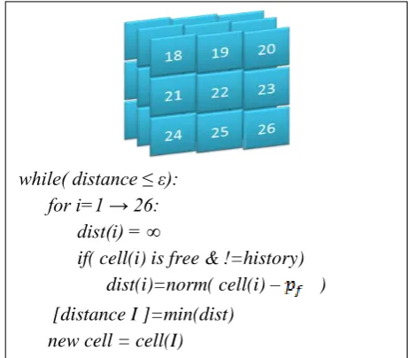
The same algorithm can be extended to 3D environments by modeling the workspace as a 3D distance map where = 3. The third dimension is modeled by stacking 2D layers of cells spaced by an amount less than or equal to ε. The 26 adjacent cells are evaluated to find the nearest cell to the final configuration as shown in figure 9. In 3D, the height of the obstacle is significant since the path now can go over objects and not just around them. The performance of the algorithm in 3D is undermined by the added complexity of tripling the number of cells to evaluate at each iteration. Generally, all the three steps of computing an optimal path take significantly more time than in 2D.

Figure 9: 3D path planning algorithm.

Figure 10: Using a segmented image of the workspace to enable path planning algorithm.

1.Image segmentation

Background = 0

Foreground = x (2D) where x≠0 = height (3D)

2. Path planning

while( distance ≤ ε):

for i=1 → 26:

dist(i) = ∞

if( cell(i) is free & !=history)

dist(i)=norm( cell(i) –

)

[distance I ]=min(dist)

new cell = cell(I)

-15 -10 -5 0 5 10 15

-15 -10 -5 0 5 10 15

i=1;

for j=i+1 → length( path ):

while( line(i→j) is free):

j++

path2(i+1)=path(j-1)

0 1 2 3 4 5 6 7 8 9 10

x 105

0 0.2 0.4 0.6 0.8 ti m e t o c o m p u te i n it ia l p a th ( s e c )

# cells in grid

0 1 2 3 4 5 6 7 8 9 10

x 105

0 0.5 1 1.5 2

0 1 2 3 4 5 6 7 8 9 10

x 105

0 0.5 1 1.5 2 ti m e t o c o m p u te o p ti m a l p a th 1 ( s e c )

Figure11: Computation time grows as the size of the grid is increased. This relationship is obtained by modeling an obstacle-free workspace.

0 100 200 300 400 500 600 700 800 900 1000

0 5 10 15 20 25 30 35 # obstacles ti m e t o m o d e l w o rk s p a c e ( s e c )

Figure12: Time to map obstacles grows linearly as the number of obstacles is increased. A 60x60 grid is used to generate this plot. The time taken to map obstacles does not include the time to compute the path.

VIII. COMPUTER VISION

The main contribution of this algorithm is the improvement in the computation time needed to map a collision free path when used in sensor equipped robots by eliminating the representational cost. The digital map, an array of zeros and ones representing the workspace that this algorithm requires in order to be able to compute the distance to the final position, can be substituted by a segmented image of the workspace from the vision module. This eliminates the computation time needed to model the workspace and map the obstacles in order to generate the digital map. This is particularly important for real time path planning where the workspace is constantly changing. Figure 10 shows an example of the process of transitioning from an image to a digital map by segmentation. Figure 10 shows the image before and after segmentation where the background is now represented by zeros and the foreground by any non-zero value. This representation of the workspace is sufficient for the algorithm to be able to compute a collision free path with a minimal number of waypoints.

IX. CONCLUSION

We presented a distance transform-based algorithm for obstacle avoidance and path planning that is suitable for robots with on-board sensors. Geometric path planning is characterized by low representational cost compared to similar algorithms. Designing the algorithm around the output of the vision module can further reduce the computation time by eliminating the representational cost. Geometric path planning algorithms have their limitations when used in mobile robots since they are too local and cannot compute long paths efficiently. Doing so would require increasing the size of the grid to represent a larger region of the workspace. This represents a tradeoff between the size of the grid and the computation time. The computation cost increases as the number of cells to evaluate at each time step grows. Figure 11 shows the relationship between the time taken to compute the initial and optimal paths and the grid size. Unlike other probabilistic algorithms, the computation time is proportional to the grid size rather than the number of obstacles. Moreover, the path generated by geometric path planners clips obstacles’ corners as shown in most examples above. This represents an undesired behavior in most robot applications. Over all, geometric path planning is an efficient algorithm for localized workspaces with reasonable error margins.

REFERENCES

[1] Thrope, “path relaxation: path planning for a mobile robot.”

Proceedings of the National Conference on Artificial Intelligence,

1984.

[2] H. Moravec, “Rover visual obstacle avoidance,” Proceedings of the

Seventh International Joint Conference on Artificial Intelligence,

1981.

[3] S. Kambhampati, L. Davis, “Multiresolution path planning for mobile robots,” IEEE Journal of Robitcs and Automation, 2(3):135-145, 1986.

[4] B. Faverjon, “Obstacle avoidance using an octree in the configuration space of a manipulator,” Proceedings of IEEE International

Conference on Robotics and Automation, 1984.

[5] R. Mohring, H. Schilling, “Partitioning graphs to speed up Dijkstra’s algorithm,” ACM Journal of Experimental Algorithmics, Vol. 11, Article No. 2.8, 2006.

[6] P. Hart, N. Nilsson, B. Raphael, “A formal basis for the heuristic determination of minimum cost paths,” IEEE Transactions of System

Science and Cybernetics, Vol. ssc-4, No. 2, 1968.

[7] E. Welzl, “Constructing the visibility graph for n line segments in O(n2) time,” let.20 pp.167-171, 1985.

[8] S.M. LaValle, “Planning algorithms,” Cambridge University Press, New York, pp.228-240, 2006.

[9] L. Kavraki, J.-C. Latombe, R. Motwani, P. Raghavan, “Randomized query processing in robot path planning,” Proceedings of the 27th

Annual ACM Symposium on Theory of Computing, 1995.

[10] L. Kavraki, P. Svestka, J.-C. Latombe, M. Overmars, “Probabilistic roadmaps for path planning in high dimensional configuration spaces,”

IEEE Transactions on Robotics and Automation, 12(4), 566-580,