Auto Sizing the Transformer Network: Improving Speed, Efficiency, and Performance for Low Resource Machine Translation

Proceedings of the 3rd Workshop on Neural Generation and Translation (WNGT 2019), pages 231–240 231

Auto-Sizing the Transformer Network:

Improving Speed, E

ffi

ciency, and Performance

for Low-Resource Machine Translation

Kenton Murray Jeffery Kinnison Toan Q. Nguyen Walter Scheirer David Chiang

Department of Computer Science and Engineering University of Notre Dame

{kmurray4, jkinniso, tnguye28, walter.scheirer, dchiang}@nd.edu

Abstract

Neural sequence-to-sequence models, particu-larly the Transformer, are the state of the art in machine translation. Yet these neural networks are very sensitive to architecture and hyper-parameter settings. Optimizing these settings by grid or random search is computationally expensive because it requires many training runs. In this paper, we incorporate architecture search into a single training run through auto-sizing, which uses regularization to delete neu-rons in a network over the course of training. On very low-resource language pairs, we show that auto-sizing can improve BLEU scores by up to 3.9 points while removing one-third of the parameters from the model.

1 Introduction

Encoder-decoder based neural network models are the state-of-the-art in machine translation. How-ever, these models are very dependent on selecting optimal hyperparameters and architectures. This problem is exacerbated in very low-resource data settings where the potential to overfit is high. Un-fortunately, these searches are computationally ex-pensive. For instance,Britz et al.(2017) used over 250,000 GPU hours to compare various recurrent neural network based encoders and decoders for machine translation.Strubell et al.(2019) demon-strated the neural architecture search for a large NLP model emits over four times the carbon diox-ide relative to a car over its entire lifetime.

Unfortunately, optimal settings are highly de-pendent on both the model and the task, which means that this process must be repeated often. As a case in point, the Transformer architecture has become the best performing encoder-decoder model for machine translation (Vaswani et al., 2017), displacing RNN-based models (Bahdanau et al., 2015) along with much conventional wis-dom about how to train such models. Vaswani

et al. ran experiments varying numerous hyper-parameters of the Transformer, but only on high-resource datasets among linguistically similar lan-guages. Popel and Bojar(2018) explored ways to train Transformer networks, but only on a high-resource dataset in one language pair. Less work has been devoted to finding best practices for smaller datasets and linguistically divergent lan-guage pairs.

In this paper, we applyauto-sizing(Murray and Chiang, 2015), which is a type of architecture search conducted during training, to the Trans-former. We show that it is effective on very low-resource datasets and can reduce model size sig-nificantly, while being substantially faster than other architecture search methods. We make three main contributions.

1. We demonstrate the effectiveness of auto-sizing on the Transformer network by significantly re-ducing model size, even though the number of pa-rameters in the Transformer is orders of magnitude larger than previous natural language processing applications of auto-sizing.

2. We demonstrate the effectiveness of auto-sizing on translation quality in very low-resource set-tings. On four out of five language pairs, we ob-tain improvements in BLEU over a recommended low-resource baseline architecture. Furthermore, we are able to do so an order of magnitude faster than random search.

3. We release GPU-enabled implementations of proximal operators used for auto-sizing. Previous authors (Boyd et al.,2010;Duchi et al.,2008) have given efficient algorithms, but they don’t neces-sarily parallelize well on GPUs. Our variations are optimized for GPUs and are implemented as a general toolkit and are released as open-source software.1

2 Hyperparameter Search

While the parameters of a neural network are op-timized by gradient-based training methods, hy-perparameters are values that are typically fixed before training begins, such as layer sizes and learning rates, and can strongly influence the out-come of training. Hyperparameter optimization is a search over the possible choices of hyper-parameters for a neural network, with the objec-tive of minimizing some cost function (e.g., error, time to convergence, etc.). Hyperparameters may be selected using a variety of methods, most of-ten manual tuning, grid search (Duan and Keerthi, 2005), or random search (Bergstra and Bengio, 2012). Other methods, such as Bayesian optimiza-tion (Bergstra et al.,2011;Snoek et al.,2012), ge-netic algorithms (Benardos and Vosniakos,2007; Friedrichs and Igel,2005;Vose et al.,2019), and hypergradient updates (Maclaurin et al.,2015), at-tempt to direct the selection process based on the objective function. All of these methods require training a large number of networks with different hyperparameter settings.

In this work, we focus on a type of hyperpa-rameter optimization called auto-sizing introduced byMurray and Chiang(2015) which only requires training one network once. Auto-sizing focuses on driving groups of weights in a parameter tensor to zero through regularization. Murray and Chiang (2015) focused on the narrow case of two hidden layers in a feed-forward neural network with a rec-tified linear unit activation. In this work, we look at the broader case of all of the non-embedding pa-rameter matrices in the encoder and decoder of the Transformer network.

3 GPU Optimized Proximal Gradient

Descent

Murray and Chiang(2015) train a neural network while using a regularizer to prune units from the network, minimizing:

L=− X

f,ein data

logP(e| f;W)+λR(kWk),

whereWare the parameters of the model andRis a regularizer. For simplicity, assume that the param-eters form a single matrixW of weights. Murray

Algorithm 1Parallel`∞proximal step

Require: Vectorvwithnelements

Ensure: Decrease the largest absolute value inv

until the total decrease isηλ 1: vi ← |vi|

2: sortvin decreasing order

3: δi ←vi−vi+1,δn←vn

4: ci ← i X

i0₌₁

i0δi0 .prefix sum

5: bi = 1_i(clip_[ci−1,ci](ηλ)−ci−1)

6: pi = n X

i0_=i

bi0 .suffix sum

7: v←v−p

8: restore order and signs ofv

v1

v2

v₃

δ1=b1

δ2

b2

δ3

(a) (b)

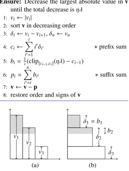
Figure 1: Illustration of Algorithm1. The shaded area, here with valueηλ = 2, represents how much the`∞ proximal step will remove from a sorted vector.

and Chiang(2015) try two regularizers:

R(W)=X

i          X j W_{i j}2

         1 2

(`2,1)

R(W)=X

i max

j |Wi j| (`∞,1)

The optimization is done using proximal gradi-ent descgradi-ent (Parikh and Boyd, 2014), which al-ternates between stochastic gradient descent steps and proximal steps:

W←W−η∇logP(e| f;w)

W←arg min W0

1

2ηkW−W

0

k2+R(W0) !

To perform the proximal step for the `∞,1 norm,

The algorithm starts by taking the absolute value of each entry and sorting the entries in de-creasing order. Figure 1a shows a histogram of sorted absolute values of an examplev. Intuitively, the goal of the algorithm is to cut a piece offthe top with areaηλ(in the figure, shaded gray).

We can also imagine the same shape as a stack of horizontal layers (Figure1b), eachiwide andδi high, with areaiδi; thenci is the cumulative area of the top ilayers. This view makes it easier to compute where the cutoffshould be. Letkbe the index such thatηλlies betweenck−1andck. Then

bi =δifori<k;bk= 1_k(ηλ−ck−1); andbi =0 for i>k. In other words,biis how much height of the ith layer should be cut off.

Finally, returning to Figure1b,piis the amount by whichvishould be decreased (the height of the gray bars). (The vector palso happens to be the projection ofvonto the`1ball of radiusηλ.)

Although this algorithm is less efficient than the quickselect-like algorithm when run in serial, the sort in line 2 and the cumulative sums in lines4 and 6 (Ladner and Fischer, 1980) can be paral-lelized to run inO(logn) passes each.

4 Transformer

The Transformer network, introduced byVaswani et al.(2017), is a sequence-to-sequence model in which both the encoder and the decoder consist of stacked self-attention layers. Each layer of the decoder can attend to the previous layer of the de-coder and the output of the ende-coder. The multi-head attention uses two affine transformations, fol-lowed by a softmax. Additionally, each layer has a position-wise feed-forward neural network (FFN) with a hidden layer of rectified linear units:

FFN(x)=W2(max(0,W1x+b1))+b2.

The hidden layer size (number of columns ofW1)

is typically four times the size of the model dimen-sion. Both the multi-head attention and the feed-forward neural network have residual connections that allow information to bypass those layers.

4.1 Auto-sizing Transformer

Though the Transformer has demonstrated re-markable success on a variety of datasets, it is highly over-parameterized. For example, the English-German WMT ’14 Transformer-base model proposed inVaswani et al.(2017) has more

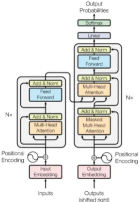
Figure 2: Architecture of the Transformer (Vaswani et al.,2017). We apply the auto-sizing method to the feed-forward (blue rectangles) and multi-head attention (orange rectangles) in all nlayers of the encoder and decoder. Note that there are residual connections that can allow information and gradients to bypass any layer we are auto-sizing.

than 60M parameters. Whereas early NMT mod-els such as Sutskever et al. (2014) have most of their parameters in the embedding layers, the added complexity of the Transformer, plus parallel developments reducing vocabulary size (Sennrich et al., 2016) and sharing embeddings (Press and Wolf,2017) has shifted the balance. Nearly 31% of the English-German Transformer’s parameters are in the attention layers and 41% in the position-wise feed-forward layers.

Accordingly, we apply the auto-sizing method to the Transformer network, and in particular to the two largest components, the feed-forward lay-ers and the multi-head attentions (blue and orange rectangles in Figure 2). A difference from the work of Murray and Chiang (2015) is that there are residual connections that allow information to bypass the layers we are auto-sizing. If the regu-larizer drives all the neurons in a layer to zero, in-formation can still pass through. Thus, auto-sizing can effectively prune out an entire layer.

4.2 Random Search

Dataset Size

Ara–Eng 234k

Fra–Eng 235k

Hau–Eng 45k

Tir–Eng 15k

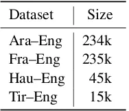
Table 1: Number of parallel sentences in training bi-texts. The French-English and Arabic-English data is from the 2017 IWSLT campaign (Mauro et al.,2012). The much smaller Hausa-English and Tigrinya-English data is from the LORELEI project.

and Bengio, 2012). In fact, Li and Talwalkar (2019) recently demonstrated that many architec-ture search methods do not beat a random baseline. In practice, randomly searching hyperparameter domains allows for an intuitive mixture of con-tinuous and categorical hyperparameters with no constraints on differentiability (Maclaurin et al., 2015) or need to cast hyperparameter values into a single high-dimensional space to predict new val-ues (Bergstra et al.,2011).

5 Experiments

All of our models are trained using the fairseq im-plementation of the Transformer (Gehring et al., 2017).2 Our GPU-optimized, proximal gradient algorithms are implemented in PyTorch and are publicly available.3 For the random hyperparame-ter search experiments, we use SHADHO,4which defines the hyperparameter tree, generates from it, and manages distributed resources (Kinnison et al.,2018). Our SHADHO driver file and modi-fications to fairseq are also publicly available.5

5.1 Settings

We looked at four different low-resource language pairs, running experiments in five directions: Arabic-English, English-Arabic, French-English, Hausa-English, and Tigrinya-English. The Ara-bic and French data comes from the IWSLT 2017 Evaluation Campaign (Mauro et al., 2012). The Hausa and Tigrinya data were provided by the LORELEI project with custom train/dev/test splits. For all languages, we tokenized and true-cased the data using scripts from Moses (Koehn et al.,2007). For the Arabic systems, we

translit-2_{https://github.com/pytorch/fairseq}

3_{https://github.com/KentonMurray/ProxGradPytorch} 4_{https://github.com/jeffkinnison/shadho}

5_{https://bitbucket.org/KentonMurray/fairseq autosizing}

erated the data using the Buckwalter translitera-tion scheme. All of our systems were run us-ing subword units (BPE) with 16,000 merge op-erations on concatenated source and target train-ing data (Sennrich and Haddow, 2016). We clip norms at 0.1, use label smoothed cross-entropy with value 0.1, and an early stopping criterion when the learning rate is smaller than 10−5. All of our experiments were done using the Adam opti-mizer (Kingma and Ba,2015), a learning rate of 10−4, and dropout of 0.1. At test time, we de-coded using a beam of 5 with length normalization (Boulanger-Lewandowski et al.,2013) and evalu-ate using case-sensitive, detokenized BLEU ( Pap-ineni et al.,2002).

5.1.1 Baseline

The originally proposed Transformer model is too large for our data size – the model will overfit the training data. Instead, we use the recommended settings in fairseq for IWSLT German-English as a baseline since two out of our four language pairs are also from IWSLT. This architecture has 6 lay-ers in both the encoder and decoder, each with 4 attention heads. Our model dimension isdmodel = 512, and our FFN dimension is 1024.

5.1.2 Auto-sizing parameters

Auto-sizing is implemented as two different types of group regularizers, `2,1 and `∞,1. We apply

the regularizers to the feed-forward network and multi-head attention in each layer of the encoder and decoder. We experiment across a range of reg-ularization coefficient values, λ, that control how large the regularization proximal gradient step will be. We note that different regularization coeffi -cient values are suited for different types or reg-ularizers. Additionally, all of our experiments use the same batch size, which is also related toλ.

5.1.3 Random search parameters

vary-ing our samples over{512,1024,2048}. This too differs from most Transformer implementations, which have identical layer hyperparameters.

5.2 Auto-sizing vs. Random Search

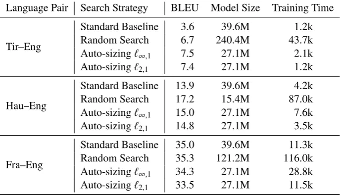
Table 2 compares the performance of random search with auto-sizing across, BLEU scores, model size, and training times. The baseline sys-tem, the recommended IWSLT setting in fairseq, has almost 40 million parameters. Auto-sizing the feed-forward network sub-components in each layer of this baseline model with `2,1 = 10.0 or

`∞,1 = 100.0 removes almost one-third of the

to-tal parameters from the model. For Hausa-English and Tigrinya-English, this also results in substan-tial BLEU score gains, while only slightly hurt-ing performance for French-English. The BLEU scores for random search beats the baseline for all language pairs, but auto-sizing still performs best on Tigrinya-English – even with 72 different, ran-dom hyperparameter configurations.

Auto-sizing trains in a similar amount of time to the baseline system, whereas the cumulative train-ing time for all of the models in random search is substantially slower. Furthermore, for Tigrinya-English and French-Tigrinya-English, random search found models that were almost 10 and 5 times larger re-spectively than the auto-sized models.

5.3 Training times

One of the biggest downsides of searching over architectures using a random search process is that it is very time and resource expensive. Contrary to that, auto-sizing relies on only trainingonemodel. Auto-sizing relies on a proximal gradient step after a standard gradient descent step. However, the addition of these steps for our two group reg-ularizers does not significantly impact training times. Table 3 shows the total training time for both `2,1 = 0.1 and `∞,1 = 0.5. Even with the

extra proximal step, auto-sizing using`2,1actually

converges faster on two of the five language pairs. Note that these times are for smaller regularization coefficients. Larger coefficients will cause more values to go to zero, which will make the model converge faster.

5.4 Auto-sizing Sub-Components

As seen above, on very low-resource data, auto-sizing is able to quickly learn smaller, yet better, models than the recommended low-resource trans-former architecture. Here, we look at the impact

of applying auto-sizing to various sub-components of the Transformer network. In section 3, fol-lowing the work of Murray and Chiang (2015), auto-sizing is described as intelligently applying a group regularizer to our objective function. The relative weight, or regularization coefficient, is a hyperparameter defined asλ. In this section, we also look at the impact of varying the strength of this regularization coefficient.

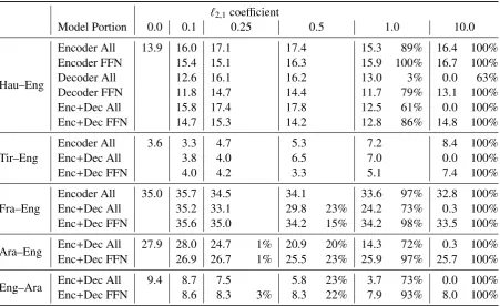
Tables 4 and 5 demonstrate the impact of varying the regularization coefficient strength has on BLEU scores and model size across various model sub-components. Recall that each layer of the Transformer network has multi-head attention components and a feed-forward network sub-component. We denote experiments only apply-ing auto-sizapply-ing to feed-forward network as “FFN”. We also experiment with auto-sizing the multi-head attention in conjunction with the FFN, which we denote “All”. A regularization coefficient of 0.0 refers to the baseline model without any auto-sizing. Columns which contain percentages re-fer to the number of rows in a PyTorch parameter that auto-sizing was applied to, that were entirely driven to zero. In effect, neurons deleted from the model. Note that individual values in a row may be zero, but if even a single value remains, infor-mation can continue to flow through this and it is not counted as deleted. Furthermore, percentages refer only to the parameters that auto-sizing was applied to, not the entire model. As such, with the prevalence of residual connections, a value of 100% does not mean the entire model was deleted, but merely specific parameter matrices. More spe-cific experimental conditions are described below.

5.4.1 FFN matrices and multi-head attention

Rows corresponding to “All” in tables4and5look at the impact of varying the strength of both the `∞,1 and `2,1 regularizers across all learned

pa-rameters in the encoder and decoders (multi-head and feed-forward network parameters). Using`∞,1

regularization (table5), auto-sizing beats the base-line BLEU scores on three language pairs: Hau– Eng, Tir–Eng, Fra–Eng. However, BLEU score improvements only occur on smaller regulariza-tion coefficients that do not delete model portions. Looking at`2,1regularization across all learned

Language Pair Search Strategy BLEU Model Size Training Time

Tir–Eng

Standard Baseline 3.6 39.6M 1.2k

Random Search 6.7 240.4M 43.7k

Auto-sizing`∞,1 7.5 27.1M 2.1k

Auto-sizing`2,1 7.4 27.1M 1.2k

Hau–Eng

Standard Baseline 13.9 39.6M 4.2k

Random Search 17.2 15.4M 87.0k

Auto-sizing`∞,1 15.0 27.1M 7.6k

Auto-sizing`2,1 14.8 27.1M 3.5k

Fra–Eng

Standard Baseline 35.0 39.6M 11.3k

Random Search 35.3 121.2M 116.0k

Auto-sizing`∞,1 34.3 27.1M 28.8k

Auto-sizing`2,1 33.5 27.1M 11.5k

Table 2: Comparison of BLEU scores, model size, and training time on Tigrinya-English, Hausa-English, and French-English. Model size is the total number of parameters. Training time is measured in seconds. Baseline is the recommended low-resource architecture in fairseq. Random search represents the best model found from 72 (Tigrinya), 40 (Hausa), and 10 (French) different randomly generated architecture hyperparameters. Both auto-sizing methods, on both languages, start with the exact same initialization and number of parameters as the baseline, but converge to much smaller models across all language pairs. On the very low-resource languages of Hausa and Tigrinya auto-sizing finds models with better BLEU scores. Random search is eventually able to find better models on French and Hausa, but is an order of magnitude slower.

Language Pair Baseline `2,1 `∞,1

Fra–Eng 11.3k 11.5k 28.8k

Ara–Eng 15.1k 16.6k 40.8k

Eng–Ara 16.6k 11.0k 21.9k

Hau–Eng 4.2k 3.5k 7.6k

Tir–Eng 1.2k 1.2k 2.1k

Table 3: Overall training times in seconds on a Nvidia GeForce GTX 1080Ti GPU for small regularization values. Note that high regularization values will delete too many values and cause training to end sooner. In general, `2,1 regularization does not appreciably slow down training, but`∞,1can be twice as slow. Per epoch, roughly the same ratios in training times hold.

regularization coefficients, and stronger regulariz-ers that delete parts of the model hurt translation quality. Multi-head attention is an integral portion of the Transformer model and auto-sizing this gen-erally leads to performance hits.

5.4.2 FFN matrices

As the multi-head attention is a key part of the Transformer, we also looked at auto-sizing just the feed-forward sub-component in each layer of the encoder and decoder. Rows deonted by “FFN” in tables 4and5 look at applying auto-sizing to all

of the feed-forward network sub-components of the Transformer, but not to the multi-head atten-tion. With`∞,1 regularization, we see BLEU

im-provements on four of the five language pairs. For both Hausa-English and Tigrinya-English, we see improvements even after deleting all of the feed-forward networks in all layers. Again, the resid-ual connections allow information to flow around these sub-components. Using `2,1 regularization,

we see BLEU improvements on three of the lan-guage pairs. Hausa-English and Tigrinya-English maintain a BLEU gain even when deleting all of the feed-forward networks.

Auto-sizing only the feed-forward sub-component, and not the multi-head attention part, results in better BLEU scores, even when deleting all of the feed-forward network components. Impressively, this is with a model that has fully one-third fewer parameters in the encoder and decoder layers. This is beneficial for faster inference times and smaller disk space.

5.4.3 Encoder vs. Decoder

In table4, experiments on Hau-Eng look at the im-pact of auto-sizing either the encoder or the de-coder separately. Applying a strong enough regu-larizer to delete portions of the model (`2,1 ≥1.0)

`2,1coefficient

Model Portion 0.0 0.1 0.25 0.5 1.0 10.0

Hau–Eng

Encoder All 13.9 16.0 17.1 17.4 15.3 89% 16.4 100%

Encoder FFN 15.4 15.1 16.3 15.9 100% 16.7 100%

Decoder All 12.6 16.1 16.2 13.0 3% 0.0 63%

Decoder FFN 11.8 14.7 14.4 11.7 79% 13.1 100%

Enc+Dec All 15.8 17.4 17.8 12.5 61% 0.0 100%

Enc+Dec FFN 14.7 15.3 14.2 12.8 86% 14.8 100%

Tir–Eng

Encoder All 3.6 3.3 4.7 5.3 7.2 8.4 100%

Enc+Dec All 3.8 4.0 6.5 7.0 0.0 100%

Enc+Dec FFN 4.0 4.2 3.3 5.1 7.4 100%

Fra–Eng

Encoder All 35.0 35.7 34.5 34.1 33.6 97% 32.8 100%

Enc+Dec All 35.2 33.1 29.8 23% 24.2 73% 0.3 100%

Enc+Dec FFN 35.6 35.0 34.2 15% 34.2 98% 33.5 100%

Ara–Eng Enc+Dec All 27.9 28.0 24.7 1% 20.9 20% 14.3 72% 0.3 100%

Enc+Dec FFN 26.9 26.7 1% 25.5 23% 25.9 97% 25.7 100%

Eng–Ara Enc+Dec All 9.4 8.7 7.5 5.8 23% 3.7 73% 0.0 100%

Enc+Dec FFN 8.6 8.3 3% 8.3 22% 7.9 93% 8.0 100%

Table 4: BLEU scores and percentage of parameter rows deleted by auto-sizing on various sub-components of the model, across varying strengths of`2,1 regularization. 0.0 refers to the baseline without any regularizer. Blank spaces mean less than 1% of parameters were deleted. In the two very low-resource language pairs (Hausa-English and Tigrinya-English), deleting large portions of the encoder can actually help performance. However, deleting the decoder hurts performance.

`∞,1

0.0 0.1 0.25 0.5 1.0 10.0 100.0

Hau–Eng Enc+Dec All 13.9 15.5 14.7 16.0 16.7 14.9 4% 1.5 100% Enc+Dec FFN 13.4 14.3 14.1 12.9 15.3 0% 15.0 100%

Tir–Eng Enc+Dec All 3.6 4.6 3.4 3.4 3.7 7.4 0% 2.4 100%

Enc+Dec FFN 3.6 3.8 3.9 3.6 4.7 0% 7.5 100%

Fra–Eng Enc+Dec All 35.0 35.2 35.4 34.9 35.3 26.3 13% 1.7 100% Enc+Dec FFN 34.8 35.5 35.4 35.0 34.1 0% 34.3 100%

Ara–Eng Enc+Dec All 27.9 27.3 27.5 27.6 26.9 18.5 22% 0.6 100% Enc+Dec FFN 27.8 27.2 28.3 27.6 25.4 0% 25.4 100%

Eng–Ara Enc+Dec All 9.4 9.1 8.3 8.4 8.7 5.2 25% 0.6 100%

Enc+Dec FFN 8.8 9.2 9.0 8.9 8.2 0% 8.3 100%

FFN”) results in a BLEU score drop. However, ap-plying auto-sizing to only the encoder (“Encoder All” and “Encoder FFN”) yields a BLEU gain while creating a smaller model. Intuitively, this makes sense as the decoder is closer to the out-put of the network and requires more modeling ex-pressivity.

In addition to Hau–Eng, table 4 also con-tains experiments looking at auto-sizing all sub-components of all encoder layers of Tir–Eng and Fra–Eng. For all three language pairs, a small reg-ularization coefficient for the `2,1 regularizer

ap-plied to the encoder increases BLEU scores. How-ever, no rows are driven to zero and the model size remains the same. Consistent with Hau–Eng, us-ing a larger regularization coefficient drives all of the encoder’s weights to all zeros. For the smaller Hau–Eng and Tir–Eng datasets, this actually re-sults in BLEU gains over the baseline system. Sur-prisingly, even on the Fra–Eng dataset, which has more than 15x as much data as Tir–Eng, the per-formance hit of deleting the entire encoder was only 2 BLEU points.

Recall from Figure 2 that there are residual connections that allow information and gradients to flow around both the multi-head attention and feed-forward portions of the model. Here, we have the case that all layers of the encoder have been completely deleted. However, the decoder still at-tends over the source word and positional embed-dings due to the residual connections. We hypoth-esize that for these smaller datasets that there are too many parameters in the baseline model and over-fitting is an issue.

5.5 Random Search plus Auto-sizing

Above, we have demonstrated that auto-sizing is able to learn smaller models, faster than random search, often with higher BLEU scores. To com-pare whether the two architecture search algo-rithms (random and auto-sizing) can be used in conjunction, we also looked at applying both`2,1

and`∞,1regularization techniques to the FFN

net-works in all encoder and decoder layers during random search. In addition, this looks at how ro-bust the auto-sizing method is to different initial conditions.

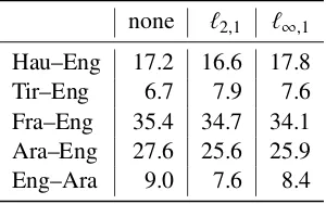
For a given set of hyperparameters generated by the random search process, we initialize three identicalmodels and train a baseline as well as one with each regularizer (`2,1=1.0 and`∞,1=10.0).

none `2,1 `∞,1

Hau–Eng 17.2 16.6 17.8

Tir–Eng 6.7 7.9 7.6

Fra–Eng 35.4 34.7 34.1

Ara–Eng 27.6 25.6 25.9

Eng–Ara 9.0 7.6 8.4

Table 6: Test BLEU scores for the models with the best dev perplexity found using random search over num-ber of layers and size of layers. Regularization values of`2,1 =1.0 and`∞,1 =10.0 were chosen based on ta-bles4and5as they encouraged neurons to be deleted. For the very low-resource language pairs, auto-sizing helped in conjunction with random search.

We trained 216 Tir–Eng models (3 · 72 hyper-parameter config.), 120 Hau–Eng, 45 Ara–Eng, 45 Eng–Ara, and 30 Fra–Eng models. Using the model with the best dev perplexity found during training, table 6 shows the test BLEU scores for each of the five language pairs. For the very low-resource language pairs of Hau–Eng and Tir–Eng, auto-sizing is able to find the best BLEU scores.

6 Conclusion

In this paper, we have demonstrated the eff ective-ness of auto-sizing on the Transformer network. On very low-resource datasets, auto-sizing was able to improve BLEU scores by up to 3.9 points while simultaneously deleting one-third of the pa-rameters in the encoder and decoder layers. This was accomplished while being significantly faster than other search methods.

Additionally, we demonstrated how to apply proximal gradient methods efficiently using a GPU. Previous work on optimizing proximal gra-dient algorithms serious impacts speed perfor-mance when the computations are moved offof a CPU and parallelized. Leveraging sorting and pre-fix summation, we reformulated these methods to be GPU efficient.

Acknowledgements

This research was supported in part by Univer-sity of Southern California, subcontract 67108176 under DARPA contract HR0011-15-C-0115. We would like to thank Justin DeBenedetto for help-ful comments.

References

Dzmitry Bahdanau, Kyunghyun Cho, and Yoshua Ben-gio. 2015. Neural machine translation by jointly learning to align and translate. InProc. ICLR.

P. G. Benardos and G.-C. Vosniakos. 2007. Optimiz-ing feedforward artificial neural network architec-ture. Engineering Applications of Artificial Intelli-gence, 20:365–382.

James Bergstra and Yoshua Bengio. 2012. Random search for hyper-parameter optimization. Journal of Machine Learning Research, 13:281–305.

James S. Bergstra, R´emi Bardenet, Yoshua Bengio, and Bal´azs K´egl. 2011. Algorithms for hyper-parameter optimization. In Advances in Neural Information Processing Systems, pages 2546–2554.

Nicolas Boulanger-Lewandowski, Yoshua Bengio, and Pascal Vincent. 2013. Audio chord recognition with recurrent neural networks. In Proc. International Society for Music Information Retrieval, pages 335– 340.

Stephen Boyd, Neal Parikh, Eric Chu, Borja Peleato, and Jonathan Eckstein. 2010. Distributed optimiza-tion and statistical learning via the alternating direc-tion method of multipliers. Foundations and Trends in Machine learning, 3(1):1–122.

Denny Britz, Anna Goldie, Minh-Thang Luong, and Quoc Le. 2017. Massive exploration of neural ma-chine translation architectures. In Proc. EMNLP, pages 1442–1451.

Kai-Bo Duan and S. Sathiya Keerthi. 2005. Which is the best multiclass SVM method? An empirical study. InInternational Workshop on Multiple Clas-sifier Systems, pages 278–285.

John Duchi, Shai Shalev-Shwartz, Yoram Singer, and Tushar Chandra. 2008. Efficient projections onto the`1-ball for learning in high dimensions. InProc.

ICML, pages 272–279.

Frauke Friedrichs and Christian Igel. 2005. Evolution-ary tuning of multiple SVM parameters. Neurocom-puting, 64:107–117.

Jonas Gehring, Michael Auli, David Grangier, Denis Yarats, and Yann N. Dauphin. 2017. Convolutional Sequence to Sequence Learning. InProc. ICML.

Diederik P. Kingma and Jimmy Lei Ba. 2015. Adam: A method for stochastic optimization. In Proc. ICLR.

Jeffery Kinnison, Nathaniel Kremer-Herman, Douglas Thain, and Walter Scheirer. 2018. Shadho: Mas-sively scalable hardware-aware distributed hyperpa-rameter optimization. InProc. IEEE Winter Confer-ence on Applications of Computer Vision (WACV), pages 738–747.

Philipp Koehn, Hieu Hoang, Alexandra Birch, Chris Callison-Burch, Marcello Federico, Nicola Bertoldi, Brooke Cowan, Wade Shen, Christine Moran, Richard Zens, et al. 2007. Moses: Open source toolkit for statistical machine translation. InProc. ACL: Demos, pages 177–180.

Richard E. Ladner and Michael J. Fischer. 1980. Par-allel prefix computation.J. ACM, 27(4):831–838.

Liam Li and Ameet Talwalkar. 2019. Random search and reproducibility for neural architecture search.

Dougal Maclaurin, David Duvenaud, and Ryan Adams. 2015. Gradient-based hyperparameter optimization through reversible learning. InProc. ICML, pages 2113–2122.

Cettolo Mauro, Girardi Christian, and Federico Mar-cello. 2012. Wit3: Web inventory of transcribed and translated talks. InProc. EAMT, pages 261–268.

Kenton Murray and David Chiang. 2015. Auto-sizing neural networks: With applications ton-gram lan-guage models. InProc. EMNLP.

Kishore Papineni, Salim Roukos, Todd Ward, and Wei-Jing Zhu. 2002. BLEU: a method for automatic evaluation of machine translation. In Proc. ACL, pages 311–318.

Neal Parikh and Stephen Boyd. 2014. Proximal al-gorithms. Foundations and Trends in Optimization, 1(3):123–231.

Martin Popel and Ondˇrej Bojar. 2018. Training tips for the Transformer model. The Prague Bulletin of Mathematical Linguistics, 110(1):43–70.

Ofir Press and Lior Wolf. 2017. Using the output embedding to improve language models. InProc. EACL: Volume 2, Short Papers, pages 157–163.

Ariadna Quattoni, Xavier Carreras, Michael Collins, and Trevor Darrell. 2009. An efficient projection for

l1,∞regularization. InProc. ICML, pages 857–864.

Rico Sennrich and Barry Haddow. 2016. Linguistic input features improve neural machine translation. In Proc. First Conference on Machine Translation: Volume 1, Research Papers, volume 1, pages 83–91.

Jasper Snoek, Hugo Larochelle, and Ryan P. Adams. 2012. Practical Bayesian optimization of machine learning algorithms. In Advances in Neural Infor-mation Processing Systems, pages 2951–2959.

Emma Strubell, Ananya Ganesh, and Andrew McCal-lum. 2019. Energy and policy considerations for deep learning in NLP. InProc. ACL.

Ilya Sutskever, Oriol Vinyals, and Quoc V Le. 2014. Sequence to sequence learning with neural net-works. InAdvances in Neural Information Process-ing Systems, pages 3104–3112.

Ashish Vaswani, Noam Shazeer, Niki Parmar, Jakob Uszkoreit, Llion Jones, Aidan N. Gomez, Łukasz Kaiser, and Illia Polosukhin. 2017. Attention is all you need. InAdvances in Neural Information Pro-cessing Systems, pages 5998–6008.