Training Neural Network Language Models on Very Large Corpora

Training Neural Network Language Models

On Very Large Corpora

Holger Schwenk and Jean-Luc Gauvain

LIMSI-CNRS

BP 133, 91436 Orsay cedex, FRANCE

schwenk,[email protected]

Abstract

During the last years there has been grow-ing interest in usgrow-ing neural networks for language modeling. In contrast to the well known back-offn-gram language models, the neural network approach attempts to overcome the data sparseness problem by performing the estimation in a continuous space. This type of language model was mostly used for tasks for which only a very limited amount of in-domain training data is available.

In this paper we present new algorithms to train a neural network language model on very large text corpora. This makes pos-sible the use of the approach in domains where several hundreds of millions words of texts are available. The neural network language model is evaluated in a state-of-the-art real-time continuous speech recog-nizer for French Broadcast News. Word error reductions of 0.5% absolute are re-ported using only a very limited amount of additional processing time.

1 Introduction

Language models play an important role in many applications like character and speech recognition, machine translation and information retrieval. Sev-eral approaches have been developed during the last

∗

This work was partially financed by the European Commis-sion under the FP6 Integrated Project TC-STAR.

decades like n-gram back-off word models (Katz, 1987), class models (Brown et al., 1992), structured language models (Chelba and Jelinek, 2000) or max-imum entropy language models (Rosenfeld, 1996). To the best of our knowledge word and classn-gram back-off language models are still the dominant ap-proach, at least in applications like large vocabulary continuous speech recognition or statistical machine translation. In many publications it has been re-ported that modified Kneser-Ney smoothing (Chen and Goodman, 1999) achieves the best results. All the reference back-off language models (LM) de-scribed in this paper are build with this technique, using the SRI LM toolkit (Stolcke, 2002).

The field of natural language processing has re-cently seen some changes by the introduction of new statistical techniques that are motivated by success-ful approaches from the machine learning commu-nity, in particular continuous space LMs using neu-ral networks (Bengio and Ducharme, 2001; Bengio et al., 2003; Schwenk and Gauvain, 2002; Schwenk and Gauvain, 2004; Emami and Jelinek, 2004), dom Forest LMs (Xu and Jelinek, 2004) and Ran-dom cluster LMs (Emami and Jelinek, 2005). Usu-ally new approaches are first verified on small tasks using a limited amount of LM training data. For instance, experiments have been performed using the Brown corpus (1.1M words), parts of the Wall-street journal corpus (19M words) or transcriptions of acoustic training data (up to 22M words). It is much more challenging to compare the new statis-tical techniques to carefully optimized back-off LM trained on large amounts of data (several hundred millions words). Training may be difficult and very

time consuming and the algorithms used with sev-eral tens of millions examples may be impracticable for larger amounts. Training back-off LMs on large amounts of data is not a problem, as long as power-ful machines with enough memory are available in order to calculate the word statistics. Practice has also shown that back-off LMs seem to perform very well when large amounts of training data are avail-able and it is not clear that the above mentioned new approaches are still of benefit in this situation.

In this paper we compare the neural network language model to n-gram model with modified Kneser-Ney smoothing using LM training corpora of up to 600M words. New algorithms are pre-sented to effectively train the neural network on such amounts of data and the necessary capacity is ana-lyzed. The LMs are evaluated in a real-time state-of-the-art speech recognizer for French Broadcast News. Word error reductions of up to 0.5% abso-lute are reported.

2 Architecture of the neural network LM

The basic idea of the neural network LM is to project the word indices onto a continuous space and to use a probability estimator operating on this space (Ben-gio and Ducharme, 2001; Ben(Ben-gio et al., 2003). Since the resulting probability functions are smooth func-tions of the word representation, better generaliza-tion to unknownn-grams can be expected. A neural network can be used to simultaneously learn the pro-jection of the words onto the continuous space and to estimate then-gram probabilities. This is still a

n-gram approach, but the LM posterior probabilities are ”interpolated” for any possible context of length

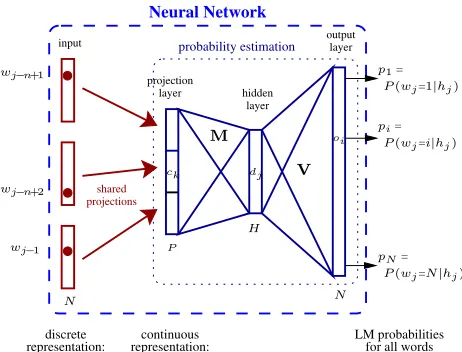
n-1 instead of backing-off to shorter contexts. The architecture of the neural network n-gram LM is shown in Figure 1. A standard fully-connected multi-layer perceptron is used. The inputs to the neural network are the indices of the n−1 previous words in the vocabulary hj =

wj−n+1, ..., wj−2, wj−1and the outputs are the

pos-terior probabilities of all words of the vocabulary:

P(wj =i|hj) ∀i∈[1, N] (1)

where N is the size of the vocabulary. The input uses the so-called 1-of-n coding, i.e., the i-th word of the vocabulary is coded by setting the i-th ele-ment of the vector to 1 and all the other eleele-ments to

projection

layer hidden layer

output layer input

projectionsshared

continuous representation: representation: indices in wordlist

LM probabilities discrete

for all words

probability estimation

Neural Network

N

wj−1 P

H

N

P(wj=1|hj) wj−n+1

wj−n+2

P(wj=i|hj)

P(wj=N|hj)

Pdimensional vectors

ck

oi

M

V

dj

p1=

pN= pi=

Figure 1: Architecture of the neural network language model. hj denotes the context

wj−n+1, ..., wj−1. P is the size of one

projec-tion and H and N is the size of the hidden and output layer respectively. When shortlists are used the size of the output layer is much smaller then the size of the vocabulary.

0. The i-th line of theN×Pdimensional projection matrix corresponds to the continuous representation of thei-th word. Let us denoteckthese projections,

dj the hidden layer activities,oithe outputs,pitheir softmax normalization, andmjl, bj, vij andki the hidden and output layer weights and the correspond-ing biases. Uscorrespond-ing these notations the neural network performs the following operations:

dj = tanh X

l

mjlcl+bj !

(2)

oi = X

j

vijdj+ki (3)

pi = eoi / N X

k=1

eok ₍₄₎

The value of the output neuronpi corresponds di-rectly to the probabilityP(wj =i|hj). Training is performed with the standard back-propagation algo-rithm minimizing the following error function:

E=

N X

i=1

tilog pi+β( X

jl

m2_jl+X

ij

v2_ij) (5)

sentence and 0.0 for all the other ones. The first part of this equation is the cross-entropy between the out-put and the target probability distributions, and the second part is a regularization term that aims to pre-vent the neural network from overfitting the training data (weight decay). The parameterβ has to be de-termined experimentally.

It can be shown that the outputs of a neural net-work trained in this manner converge to the posterior probabilities. Therefore, the neural network directly minimizes the perplexity on the training data. Note also that the gradient is back-propagated through the projection-layer, which means that the neural net-work learns the projection of the words onto the con-tinuous space that is best for the probability estima-tion task. The complexity to calculate one probabil-ity with this basic version of the neural network LM is quite high:

O = (n−1)×P×H+H+H×N +N (6)

wherePis the size of one projection andHandNis the size of the hidden and output layer respectively. Usual values aren=4,P=50 to 200,H=400 to 1000 andN=40k to 200k. The complexity is dominated by the large size of the output layer. In this paper the improvements described in (Schwenk, 2004) have been used:

1. Lattice rescoring: speech recognition is done with a standard back-off LM and a word lattice is generated. The neural network LM is then used to rescore the lattice.

2. Shortlists: the neural network is only used to predict the LM probabilities of a subset of the whole vocabulary.

3. Regrouping: all LM probabilities needed for one lattice are collected and sorted. By these means all LM probability requests with the same contextht lead to only one forward pass through the neural network.

4. Block mode: several examples are propagated at once through the neural network, allowing the use of faster matrix/matrix operations.

5. CPU optimization: machine specific BLAS libraries are used for fast matrix and vector op-erations.

The idea behind shortlists is to use the neural network only to predict thesmost frequent words,

s |V|, reducing by these means drastically the complexity. All words of the word list are still con-sidered at the input of the neural network. The LM probabilities of words in the shortlist (PˆN) are cal-culated by the neural network and the LM probabil-ities of the remaining words (PˆB) are obtained from a standard4-gram back-off LM:

ˆ

P(wt|ht) = (

ˆ

PN(wt|ht)PS(ht) ifwt∈shortlist

ˆ

PB(wt|ht) else

(7)

PS(ht) = X

w∈shortlist(ht)

ˆ

PB(w|ht) (8)

It can be considered that the neural network redis-tributes the probability mass of all the words in the shortlist. This probability mass is precalculated and stored in the data structures of the back-off LM. A back-off technique is used if the probability mass for a requested input context is not directly available.

Normally, the output of a speech recognition sys-tem is the most likely word sequence given the acoustic signal, but it is often advantageous to pre-serve more information for subsequent processing steps. This is usually done by generating a lattice, a graph of possible solutions where each arc cor-responds to a hypothesized word with its acoustic and language model scores. In the context of this work LIMSI’s standard large vocabulary continuous speech recognition decoder is used to generate lat-tices using an-gram back-off LM. These lattices are then processed by a separate tool and all the LM probabilities on the arcs are replaced by those calcu-lated by the neural network LM. During this lattice rescoring LM probabilities with the same contextht are often requested several times on potentially dif-ferent nodes in the lattice. Collecting and regrouping all these calls prevents multiple forward passes since all LM predictions for the same context are immedi-ately available at the output.

Math Kernel Library was used.1 Bunch mode is also used for training the neural network. Training of a typical network with a hidden layer with 500 nodes and a shortlist of length 2000 (about 1M parameters) take less than one hour for one epoch through four million examples on a standard PC.

3 Application to Speech Recognition

In this paper the neural network LM is evaluated in a real-time speech recognizer for French Broad-cast News. This is a very challenging task since the incorporation of the neural network LM into the speech recognizer must be very effective due to the time constraints. The speech recognizer it-self runs in 0.95xRT2and the neural network in less than 0.05xRT. The compute platform is an Intel Pen-tium 4 extreme (3.2GHz, 4GB RAM) running Fe-dora Core 2 with hyper-threading.

The acoustic model uses tied-state position-dependent triphones trained on about 190 hours of Broadcast News data. The speech features consist of 39 cepstral parameters derived from a Mel fre-quency spectrum estimated on the 0-8kHz band (or 0-3.8kHz for telephone data) every 10ms. These cepstral coefficients are normalized on a segment cluster basis using cepstral mean removal and vari-ance normalization. The feature vectors are linearly transformed (MLLT) to better fit the diagonal co-variance Gaussians used for acoustic modeling.

Decoding is performed in two passes. The first fast pass generates an initial hypothesis, followed by acoustic model adaptation (CMLLR and MLLR) and a second decode pass using the adapted mod-els. Each pass generates a word lattice which is ex-panded with a 4-gram LM. The best solution is then extracted using pronunciation probabilities and con-sensus decoding. Both passes use very tight prun-ing thresholds, especially for the first pass, and fast Gaussian computation based on Gaussian short lists. For the final decoding pass, the acoustic models include 23k position-dependent triphones with 12k tied states, obtained using a divisive decision tree based clustering algorithm with a 35 base phone set.

1_{http://www.intel.com/software/products/mkl/}

2_{In speech recognition, processing time is measured in}

mul-tiples of the length of the speech signal, the real time factor xRT. For a speech signal of 2h, a processing time of 0.5xRT corresponds to 1h of calculation.

The system is described in more detail in (Gauvain et al., 2005).

The neural network LM is used in the last pass to rescore the lattices. A short-list of length 8192 was used in order to fulfill the constraints on the pro-cessing time (the complexity of the neural network to calculate a LM probability is almost linear with the length of the short-list). This gives a coverage of about 85% when rescoring the lattices, i.e. the per-centage of LM requests that are actually performed by the neural network.

3.1 Language model training data

The following resources have been used for lan-guage modeling:

• Transcriptions of the acoustic training data (4.0M words)

• Commercial transcriptions (88.5M words)

• Newspaper texts (508M words)

• WEB data (13.6M words)

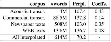
First a language model was built for each cor-pus using modified Kneser-Ney smoothing as imple-mented in the SRI LM toolkit (Stolcke, 2002). The individual LMs were then interpolated and merged together. An EM procedure was used to determine the coefficients that minimize the perplexity on the development data. Table 1 summarizes the charac-teristics of the individual text corpora.

corpus #words Perpl. Coeffs.

Acoustic transcr. 4M 107.4 0.43

Commercial transcr. 88.5M 137.8 0.14

Newspaper texts 508M 103.0 0.35

WEB texts 13.6M 136.7 0.08

All interpolated 614M 70.2

-Table 1: Characteristics of the text corpora (number of words, perplexity on the development corpus and interpolation coefficients)

the newspaper and WEB texts reflect less well the speaking style of broadcast news, but this is to some extent counterbalanced by the large amount of data. One could say that these texts are helpful to learn the general grammar of the language. The word list includes 65301 words and the OOV rate is 0.95% on a development set of 158k words.

3.2 Training on in-domain data only

Following the above discussion, it seems natural to first train a neural network LM on the transcrip-tions of the acoustic data only. The architecture of the neural network is as follows: a continuous word representation of dimension 50, one hidden layer with 500 neurons and an output layer limited to the 8192 most frequent words. This results in 3.2M parameters for the continuous representation of the words and about 4.2M parameters for the sec-ond part of the neural network that estimates the probabilities. The network is trained using standard stochastic back-propagation.3 The learning rate was set to0.005with an exponential decay and the regu-larization term is weighted with0.00003. Note that fast training of neural networks with more than 4M parameters on 4M examples is already a challenge. The same fast algorithms as described in (Schwenk, 2004) were used. Apparent convergence is obtained after about 40 epochs though the training data, each one taking 2h40 on standard PC equipped with two Intel Xeon 2.8GHz CPUs.

The neural network LM alone achieves a perplex-ity of 103.0 which is only a 4% relative reduction with respect to the back-off LM (107.4, see Table 1). If this neural network LM is interpolated with the back-off LM trained on the whole training set the perplexity decreases from 70.2 to 67.6. Despite this small improvements in perplexity a notable word er-ror reduction was obtained from 14.24% to 14.02%, with the lattice rescoring taking less than 0.05xRT. In the following sections, it is shown that larger im-provements can be obtained by training the neural network on more data.

3.3 Adding selected data

Training the neural network LM with stochastic back-propagation on all the available text corpora

3_{The weights are updated after each example.}

would take quite a long time. The estimated time for one training epoch with the 88M words of com-mercial transcriptions is 58h, and more than 12 days if all the 508M words of newspaper texts were used. This is of course not very practicable. One solution to this problem is to select a subset of the data that seems to be most useful for the task. This was done by selecting six month of the commercial transcrip-tions that minimize the perplexity on the develop-ment set. This gives a total of 22M words and the training time is about 14h per epoch.

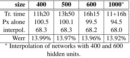
One can ask if the capacity of the neural network should be augmented in order to deal with the in-creased number of examples. Experiments with hid-den layer sizes from 400 to 1000 neurons have been performed (see Table 2).

size 400 500 600 1000∗ Tr. time 11h20 13h50 16h15 11+16h

Px alone 100.5 100.1 99.5 94.5

interpol. 68.3 68.3 68.2 68.0

Werr 13.99% 13.97% 13.96% 13.92%

∗_{Interpolation of networks with 400 and 600}

hidden units.

Table 2: Performance for a neural network LM and training time per epoch as a function of the size of the hidden layer (fixed 6 months subset of commer-cial transcripts).

Although there is a small decrease in perplexity and word error when increasing the dimension of the hidden layer, this is at the expense of a higher pro-cessing time. The training and recognition time are in fact almost linear to the size of the hidden layer. An alternative approach to augment the capacity of the neural network is to modify the dimension of the continuous representation of the words (in the range 50 to 150). The idea behind this is that the proba-bility estimation may be easier in a higher dimen-sional space (instead of augmenting the capacity of the non-linear probability estimator itself). This is similar in spirit to the theory behind support vector machines (Vapnik, 1998).

90 95 100 105 110 115 120

0 10 20 30 40 50

Perplexity

Epochs

dim 50 dim 60 dim 70 dim 100 dim 120 dim 150

Figure 2: Perplexity in function of the size of the continuous word representation (500 hidden units, fixed 6 months subset of commercial transcripts).

hidden layer is increased. Second, convergence is faster: the best result is obtained after about 15 epochs while up to 40 are needed with large hidden layers. Finally, increasing the size of the continu-ous word representation has only a small effect on the training and recognition complexity of the neu-ral network4 _{since most of the calculation is done}

to propagate and learn the connections between the hidden and the output layer (see equation 6). The best result was obtained with a 120 dimensional continuous word representation. The perplexity is 67.9 after interpolation with the back-off LM and the word error rate is 13.88%.

3.4 Training on all available data

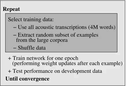
In this section an algorithm is proposed for training the neural network on arbitrary large training cor-pora. The basic idea is quite simple: instead of performing several epochs over the whole training data, a different small random subset is used at each epoch. This procedure has several advantages:

• There is no limit on the amount of training data,

• After some epochs, it is likely that all the train-ing examples have been seen at least once,

• Changing the examples after each epoch adds noise to the training procedure. This potentially increases the generalization performance.

This algorithm is summarized in figure 4. The parameters of this algorithm are the size of the ran-dom subsets that are used at each epoch. We chose

4_{14h20 forP=120 andH=500.}

80 85 90 95 100 105 110 115 120

0 5 10 15 20 25 30 35 40 45 50

Perplexity

Epochs

6 month fix 1% resampled 5% resampled 10% resampled 20% resampled

Figure 3: Perplexity when resampling different ran-dom subsets of the commercial transcriptions. (word representation of dimension 120, 500 hidden units)

to always use the full corpus of transcriptions of the acoustic data since this is the most appropriate data for the task. Experiments with different random sub-sets of the commercial transcriptions and the news-paper texts have been performed (see Figure 3 and 5). In all cases the same neural network architecture was used, i.e a 120 dimensional continuous word representation and 500 hidden units. Some experi-ments with larger hidden units showed basically the same convergence behavior. The learning rate was again set to0.005, but with a slower exponential de-cay.

First of all it can be seen from Figure 3 that the results are better when using random subsets instead of a fixed selection of 6 months, although each ran-dom subset is actually smaller (for instance a total of 12.5M examples for a subset of 10%). Best results were obtained when taking 10% of the commercial

+ Train network for one epoch Repeat

Select training data:

− Use all acoustic transcriptions (4M words) − Extract random subset of examples from the large corpora

− Shuffle data

(performing weight updates after each example) + Test performance on development data

Until convergence

Back-off LM Neural Network LM

Training data [#words] 600M 4M 22M 92.5M∗ 600M∗

Training time [h/epoch] - 2h40 14h 9h40 12h 3×12h

Perplexity (NN LM alone) - 103.0 97.5 84.0 80.0 76.5

Perplexity (interpolated LMs) 70.2 67.6 67.9 66.7 66.5 65.9

Word error rate (interpolated LMs) 14.24% 14.02% 13.88% 13.81% 13.75% 13.61%

∗_{By resampling different random parts at the beginning of each epoch.}

Table 3: Comparison of the back-off and the neural network LM using different amounts of training data. The perplexities are given for the neural network LM alone and interpolated with the back-off LM trained on all the data. The last column corresponds to three interpolated neural network LMs.

transcriptions. The perplexity is 66.7 after interpo-lation with the back-off LM and the word error rate is 13.81% (see summary in Table 3). Larger sub-sets of the commercial transcriptions lead to slower training, but don’t give better results.

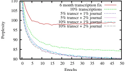
Encouraged by these results, we also included the 508M words of newspaper texts in the training data. The size of the random subsets were chosen in order to use between 4 and 9M words of each corpus. Fig-ure 5 summarizes the results. There seems to be no obvious benefit from resampling large subsets of the individual corpora. We choose to resample 10% of the commercial transcriptions and 1% of the news-paper texts.

80 85 90 95 100 105 110

0 5 10 15 20 25 30 35 40 45 50

Perplexity

Epochs

6 month transcription fix 10% transcriptions 5% transcr + 1% journal 5% transcr + 2% journal 10% transcr + 1% journal 10% transcr + 2% journal

Figure 5: Perplexity when resampling different ran-dom subsets of the commercial transcriptions and the newspaper texts.

Table 3 summarizes the results of the different neural network LMs. It can be clearly seen that the perplexity of the neural network LM alone decreases significantly with the amount of training data used. The perplexity after interpolation with the back-off LM changes only by a small amount, but there is a notable improvement in word error rate. This is

an-other experimental evidence that the perplexity of a LM is not directly related to the word error rate.

The best neural network LM achieves a word er-ror reduction of 0.5% absolute with respect to the carefully tuned back-off LM (14.24%→ 13.75%). The additional processing time needed to rescore the lattices is less than 0.05xRT. This is a significant im-provement, in particular for a fast real-time continu-ous speech recognition system. When more process-ing time is available a word error rate of 13.61% can be achieved by interpolating three neural networks together (in 0.14xRT).

3.5 Using a better speech recognizer

The experimental results have also been validated using a second speech recognizer running in about 7xRT. This systems differs from the real-time recog-nizer by a larger 200k word-list, additional acoustic model adaptation passes and less pruning. Details are described in (Gauvain et al., 2005). The word er-ror rate of the reference system using a back-off LM is 10.74%. This can be reduced to 10.51% using a neural network LM trained on the fine transcriptions only and to 10.20% when the neural network LM is trained on all data using the described resampling approach. Lattice rescoring takes about 0.2xRT.

4 Conclusions and future work

how-ever limited to a maximum of 20M words due to the high complexity of the training algorithm.

In this paper new techniques have been described to train neural network language models on large amounts of text corpora (up to 600M words). The evaluation with a state-of-the-art speech recognition system for French Broadcast News showed a signif-icant word error reduction of 0.5% absolute. The neural network LMs is incorporated into the speech recognizer by rescoring lattices. This is done in less than 0.05xRT.

Several extensions of the learning algorithm it-self are promising. We are in particular interested in smarter ways to select different subsets from the large corpus at each epoch (instead of a random choice). One possibility would be to use active learning, i.e. focusing on examples that are most useful to decrease the perplexity. One could also imagine to associate a probability to each training example and to use these probabilities to weight the random sampling. These probabilities would be up-dated after each epoch. This is similar to boosting techniques (Freund, 1995) which build sequentially classifiers that focus on examples wrongly classified by the preceding one.

5 Acknowledgment

The authors would like to thank Yoshua Bengio for fruitful discussions and helpful comments. The au-thors would like to recognize the contributions of G. Adda, M. Adda and L. Lamel for their involve-ment in the developinvolve-ment of the speech recognition systems on top of which this work is based.

References

Yoshua Bengio and Rejean Ducharme. 2001. A neural probabilistic language model. In NIPS, volume 13.

Yoshua Bengio, Rejean Ducharme, Pascal Vincent, and Christian Jauvin. 2003. A neural probabilistic lan-guage model. Journal of Machine Learning Research, 3(2):1137–1155.

Jeff Bilmes, Krste Asanovic, Chee whye Chin, and Jim Demmel. 1997. Using phipac to speed error back-propagation learning. In ICASSP, pages V:4153– 4156.

Peter F. Brown, Vincent J. Della Pietra, Peter V. deSouza, Jenifer C. Lai, and Robert L. Mercer. 1992.

Class-based n-gram models of natural language.

Computa-tional Linguistics, 18(4):467–470.

Ciprian Chelba and Frederick Jelinek. 2000. Structured language modeling. Computer Speech & Language, 13(4):283–332.

Stanley F. Chen and Joshua T. Goodman. 1999. An empirical study of smoothing techniques for language modeling. Computer Speech & Language, 13(4):359– 394.

Ahmad Emami and Frederick Jelinek. 2004. Exact train-ing of a neural syntactic language model. In ICASSP, pages I:245–248.

Ahmad Emami and Frederick Jelinek. 2005. Random clusterings for language modeling. In ICASSP, pages I:581–584.

Yoav Freund. 1995. Boosting a weak learning al-gorithm by majority. Information and Computation, 121(2):256–285.

Jean-Luc Gauvain, Gilles Adda, Martine Adda-Decker, Alexandre Allauzen, Veronique Gendner, Lori Lamel, and Holger Schwenk. 2005. Where are we in tran-scribing BN french? In Eurospeech.

Slava M. Katz. 1987. Estimation of probabilities from sparse data for the language model component of a speech recognizer. IEEE Transactions on ASSP,

35(3):400–401.

Ronald Rosenfeld. 1996. A maximum entropy approach to adaptive statistical language modeling. Computer

Speech & Language, 10(3):187–228.

Holger Schwenk and Jean-Luc Gauvain. 2002. Connec-tionist language modeling for large vocabulary contin-uous speech recognition. In ICASSP, pages I: 765– 768.

Holger Schwenk and Jean-Luc Gauvain. 2004. Neu-ral network language models for conversational speech recognition. In ICSLP, pages 1215–1218.

Holger Schwenk and Jean-Luc Gauvain. 2005. Build-ing continuous space language models for transcribBuild-ing european languages. In Eurospeech.

Holger Schwenk. 2004. Efficient training of large neu-ral networks for language modeling. In IJCNN, pages 3059–3062.

Andreas Stolcke. 2002. SRILM - an extensible language modeling toolkit. In ICSLP, pages II: 901–904.

Vladimir Vapnik. 1998. Statistical Learning Theory.

Wiley, New York.