A Numerical Approach for Modeling the Human
Upper Limb
Valentin Grecu, Nicolae Dumitru, and Luminita Grecu
Abstract— The paper presents a dynamic model
considering the human upper limb as a mechanic system with 6 degrees of freedom where the segments are moved by their own weight forces. The bones were modeled in Solid Works, the model of the upper limb obtained being very close as form to the real one. Based on this model, the calculus of mass proprieties was made. The differential equations of velocities obtained were solved using Lagrange formalism with help of Matlab programs. A dynamic model must provide a good approximation of total weight and mass distribution as well as transmissibility and amortization proprieties for bones, muscles and joints.
Index Terms —Human Joints, Human upper limb, modeling, prosthesis arm.
1. Introduction
In general, artificial limbs do not have a mechanism where patients may detect their state of functioning. This makes it very difficult to precisely detect the spatial position as well as the forces done by the prosthesis in replacement of the muscle. This problem is still more complicated when working with upper limb prosthesis, whose function is to simulate its biological equivalents (shoulder, arm, forearm, elbow, wrist and hand). All these mechanisms present a very efficient system with a lot of information (degrees of freedom, speed, angles etc) to be simulated and absorbed by brain commands. In order to carry out a functional dynamic model of the human upper limb as closely as possible to the real one, it is necessary to study the proprieties of the biological materials that make up the human body, so that the measures involved in the differential equations are as correct as possible. The experiments carried out by different researchers are based especially on models made in FEM programs.
The 3D model determination of some fundamental sizes in the study of dynamics is necessary for: improving the prosthesis and the metallic implants of the upper limb and their making in accordance with the particularities of each case.
Manuscript received March 23, 2009.
Valentin Grecu is master student with the Engineering and the Management of the Technological Systems Faculty,University of Craiova (phone: 400252205838; e-mail: valentin.grecu@ cez.ro). Dumitru Nicolae is prof.eng. PhD with the Faculty of Mechanics, University of Craiova, (e-mail: [email protected]).
Luminita Grecu is lecturer PhD with the Engineering and the Management of the Technological Systems Faculty,University of Craiova (e-mail: [email protected]).
2. Proprieties of human upper arm
The human upper arm model is composed by the segments: shoulder, arm, forearm, hand, muscles (biceps and triceps) and joints (shoulder and elbow).
The shoulder is not only a joint, but also a functional group that allows connecting the upper limb to the thorax. It can also make a great variety of motions, however, at this work, just the following motions are considered: flexing, extension, abduction and adduction. Some muscles related to the scapulohumeral joint were chosen to be studied (as shown in Table 1).This joint is classified as ball-and-socket (Figure 1), formed by an spherical surface in one of the bones and concave in another one, with 3 DOF (degrees of freedom).
The elbow has two functions:
a) flexion-extension that allows the upper limb to bend on itself or to extend;
b) pronation /supination that is, partially, the place of the motions that allow the forearm to rotate on its own axis. The joint that works in arm flexion-extension is classified as hinge and has one DOF (Figure 2). The biceps and triceps muscles (Table 2) have been selected as main participants in the flexing motions and extension of the forearm, respectively.
Fig.1 Joint ball and socket
Table 1: Shoulder Muscles
Muscle Origin Insertion Motion
Supraspinous Scapula Humerus Arm abduction Pectoralis
major Clavicle and Sternum Humerus Arm adduction Deltoid Acromio
Scapula and clavicle
Humerus Arm flexion Arm abduction Arm extension Table 2: Elbow Muscle
Muscle Origin Insertion Motion
Biceps Inferior surface of glenoid cavity scapula and coracoid process
Radius Forearm flexion
Triceps Scapula Radius Forearm
extension
To produce the motions, a set of experiments about body balance has been carried on. When the muscle exerts tension, bending the bones to sustain or to move the resistance created by the weight of the corporal segments, the muscle and the bones work mechanically as a lever. The length and the moment arm of a muscle leads to 1) affect the capacity of muscle to generate force, 2) produce joint moment, and 3) activate the motion. After calculating the moment arm, it is determined the resulting physics moment in the involved joint to determinate the motion direction. The segment weight, the segment motion and external force action can produce moment joint (Table 3). The moment is determined by multiplying the force by its arm moment. While a muscle force produces motion in a joint, the arm segment rotates, producing different moments until the equilibrium condition.
Table 3. Data of moment joint production Segment Hand Fore
arm Arm Hand Forearm Upper Arm Segment
mass/total mass
0.006 0.016 0.028 0.022 0.05
Center of mass/ length segment proximal
0.506 0.430 0.436 0.682 0.530
Center of mass/ length segment distal
0.494 0.570 0.564 0.318 0.470
3. The calculation of the moments of inertia on the 3D model of the human upper limb
Determining fundamental measurements in the study of dynamics on 3D models is necessary for perfecting prostheses and metallic implants of the upper limb and their realization according to the particularities
of each case. In order to determine the center of gravity of a component of the bony skeleton of the human upper limb and the moments of inertia, one can employ the proper command of the programs Solid Works, Mass Property, or other programs can be used, into which these files are imported, such as Pro Engineer, AutoCad, etc.
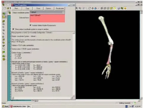
In figure 3, examples of calculation in Solid Works are presented for the various components of the human upper limb skeleton, as well as the human upper limb as a whole. For the calculation of the moments of inertia, the reference frame was placed in the component’s center of gravity.
Even though bones do not consist of a homogenous structure, the value of the mass is the one calculated with the average density: ρ = 1,3 g/cm3. Approximation leads to results that are compatible to those in literature. For the arm with muscles, the muscular density ρ= 1,14 g/cm3 was considered.
Fig.3. Calculation of mass proprieties for the human upper arm (bones).
4. The Dynamic Model of the Human Upper Limb
If we consider the upper limb’s structure as a mechanical system with 6 degrees of freedom, so that the differential equations of motion will be determined by using Lagrange’s equations:
6
..
1
=
=
∂
∂
−
⎟⎟
⎠
⎞
⎜⎜
⎝
⎛
∂
∂
i
Q
q
E
q
E
dt
d
i i c i
c
(1)c
E
– Total kinetic energy iq
- generalized variables corresponding to couples iQ
– generalized forces.The total kinetic energy is obtained:
+ ⋅ ⋅ + ⋅ ⋅ + ⋅ ⋅
= 2
3 2 2
2 1 2
1 0
2 1 2
1 2
1
q J q
J q
J
Ec z z z
6 2 5 2
5 4 2
4 3
2
1
2
1
2
1
q
J
q
J
q
J
z⋅
+
⋅
z⋅
+
⋅
z⋅
⋅
[image:2.595.41.297.519.695.2]where z0, z1, z2 represent the rotation axis corresponding to the motions of the shoulder (flexion-extension, abduction-adduction, rotation), z3 the axis corresponding to the flexion-extension motion of the elbow, z4 ,z5 the rotation axis corresponding to the motion of the wrist (flexionextension, pronation -supination) ,and 0 Z
J
, 1 ZJ
, 2 ZJ
, 3 ZJ
, 4 ZJ
, 5 ZJ
the inertia moments in connection to these axis. The following notes have been made: ul – upper limb, ra – radius, pa – palm, fi – fingers, also standing for the lengths of the afferent parts.The inertia moments in connection with the axis z0, z1, z2, z3, z4 and z5 are calculated by applying Steiner’s formulas:
J
Δ=
J
Δp+
md
2 (3)where: m –mass , d – distance between parallel axes , J - inertia moment.
fi pa IIc
z
q
m
fi
pa
J
J
⎟
+⎠
⎞
⎜
⎝
⎛
+
+
=
2 6 5 5cos
2
(4) fi pa IIc zm
fi
pa
J
J
⎟
+⎠
⎞
⎜
⎝
⎛
+
+
=
2 4 42
(5)3 2
3
3 IIc
2
pa fi raz
m
J
fi
pa
ra
J
J
⎟
+
⎠
⎞
⎜
⎝
⎛
+
+
+
=
+ (6)+ + + ⎟ ⎠ ⎞ ⎜ ⎝ ⎛ + + = IIcra J fi pa m q fi pa IIc J z J 2 5 sin 2 2 2 (7) hu IIchu ra
m
hu
J
m
q
ra
4
sin
2
2 24
⎟
+
+
⎠
⎞
⎜
⎝
⎛
+
+
+
⎟
⎠
⎞
⎜
⎝
⎛
+
+
=
IIc pa+fi IIcraz
q
m
J
fi
pa
J
J
2 5 11
2
cos
hu IIchu ra
m
hu
J
m
q
ra
4
cos
2
2 24
⎟
+
+
⎠
⎞
⎜
⎝
⎛
+
(8)+
+
⎟
⎠
⎞
⎜
⎝
⎛
+
+
=
IIc pa+fi IIcraz
m
J
fi
pa
J
J
2 0 02
(9)hu IIchu ra
m
hu
J
m
ra
2 22
2
⎟
⎠
⎞
⎜
⎝
⎛
+
+
⎟
⎠
⎞
⎜
⎝
⎛
+
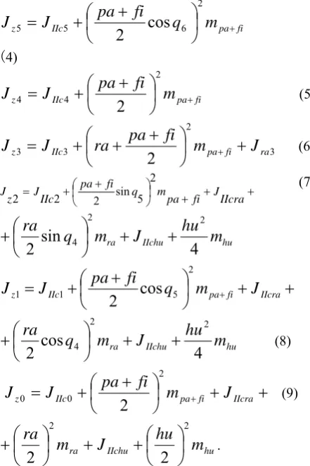
. [image:3.595.313.557.46.234.2]With the help of the Solid Works program, knowing the bone dimensions and the muscle and bone densities, these temporary figures are directly calculated by putting the reference systems directly into couples with the z axis orientated along the axis of those respective couples.
Figure 4 shows the human upper limb model for which the inertia moment calculus is made, the axis in connection to which this calculus is made, as well as the results obtained.
Fig.4. The calculus for the inertia moments for the whole arm (upper limb).
The kinetic energy derivates compared to generalized velocities and their derivates compared to time, as well as the derivates of the kinetic energy compared to the generalized coordinates become:
1 0 1
q
J
q
E
z C=
∂
∂
0
1=
∂
∂
q
E
C (10) 1 1 0q
J
q
E
dt
d
Z C⎟⎟
⎠
=
⎞
⎜⎜
⎝
⎛
∂
∂
(11) 2 1 2q
J
q
E
z C=
∂
∂
0
2=
∂
∂
q
E
C (12)2 2 2
1
q
q
J
q
E
dt
d
Z C⎟⎟
⎠
=
+
⎞
⎜⎜
⎝
⎛
∂
∂
. (13)
⎟
⎠
⎞
⎜
⎝
⎛
−
+
−
+ 5
sin
2
52
4sin
2
42
m
q
q
ra
q
q
m
fi
pa
ra fi pa 3 2 3q
J
q
E
z C=
∂
∂
0
3=
∂
∂
q
E
C (14) 3 3 32
q
q
J
q
E
dt
d
Z C⎟⎟
⎠
=
+
⎞
⎜⎜
⎝
⎛
∂
∂
. (15)
⎟
⎠
⎞
⎜
⎝
⎛
+
+
+ 5 5 4
sin
2
42
2
sin
2
m
q
q
ra
q
q
m
fi
pa
ra fi pa 4 3 4q
J
q
E
z C=
∂
∂
(16) 4 4 3q
J
q
E
dt
d
Z C⎟⎟
⎠
=
⎞
⎜⎜
⎝
⎛
∂
∂
(17)(
)
ra [image:3.595.48.269.300.631.2](
)
pa fi Cm
q
q
q
fi
pa
q
E
+
−
+
=
∂
∂
2
1
2
sin
2
2 2 2 3 5 5
(21)6 5 6
q
J
q
E
z
C
=
∂
∂
(22)
6 6
5
q
J
q
E
dt
d
Z
C
⎟⎟
⎠
=
⎞
⎜⎜
⎝
⎛
∂
∂
(23)
(
)
pa fiC
m
q
q
q
fi
pa
q
E
+
−
+
=
∂
∂
2
1
2
sin
2
2 2 2 3 6 6
(24)By replacing the equations (10)-(24) in (1), taking into account the expressions of generalized forces for i=1,6 and replacing the equations with the values for the inertia moments:
2 0
0
,
1801
kg
m
J
z=
2 1
0
,
1812
kg
m
J
z=
22
0
,
0013
kg
m
J
z=
J
z3=
0
,
0235
kg
m
22 4
0
,
0007
kg
m
J
z=
2 5
0
,
0005
kg
m
J
z=
weights:
m
pa+fi=
0
,
15
kg
,m
ra=
0
,
84
kg
,kg
m
hu=
1
,
05
,m
upper=
2
,
03
kg
and the bone sizesm
hu
=
0
,
28
,ra
=
0
,
22
m
,pa
+
fi
=
0
,
18
m
, the following differential equations system is obtained :4 5
1
1
23
,
1
cos
q
0
,
58
cos
q
7
,
18
cos
q
q
=
−
−
−
(25)−
+
=
5 2 5 2 4 42
0
.
08
q
q
sin
2
q
0
,
58
q
q
sin
2
q
q
−
−
−
0
.
63
cos
q
2cos
q
522
,
31
cos
q
1cos
q
24 2
cos
cos
78
,
69
q
q
−
(26)
5 5
3 4
4 3
3
78
.
85
q
q
sin
2
q
9
,
11
q
q
sin
2
q
q
=
−
−
(27)−
−
=
2 4 43
4
1
,
87
q
sin
2
q
58
,
21
cos
q
q
(28)4 2
2 5
1
,
87
sin
2
cos
21
,
5
q
−
q
q
−
−
−
=
2 52 5
2 3
5
7
,
87
q
sin
2
q
7
.
87
q
sin
2
q
q
(29)5
cos
48
.
193
q
−
5 5
3 4
4 3
6
10
.
8
q
q
sin
2
q
1
,
22
q
q
sin
2
q
q
=
−
−
(30)5. Solving the Differential Equation System The integration of the differential equations system that represents the reduced model of the upper limb has been made in MatLab 6.5, using the following notations:
( )
1
1
x
q
=
,q
2=
x
( )
2
,q
3=
x
( )
3
,( )
4
4
x
q
=
,q
5=
x
( )
5
,q
6=
x
( )
6
( )
7
1
x
q
=
, q2 = x( )
8 ,q
3=
x
( )
9
,( )
10
4
x
q
=
,q
5=
x
( )
11
,q
6=
x
( )
12
.On the basis of the numerical values and the articulator variables and the articulator velocities obtained as a result of integrating for
t
∈
[
0
;
0
.
5
]
and the initial conditions different from zero, the graphic representations of the motion laws and velocities corresponding to these results have been obtained (figure 5).Fig.5. Graphic diagram of the motion laws,
t
∈
[
0
;
0
,
5
]
On the basis of the numerical values and the articulator variables and the articulator velocities obtained as a result of integrating for
t
∈
[
0
;
0
,
5
]
and the initial conditions equal to zero, the graphic representations of the motion laws and velocities corresponding to these results have been obtained (figure 6).Fig.7. Graphic diagram of the motion laws and velocities,
[
0
;
0
,
4
]
∈
t
As solving of the differential equation system is numerical, the statistical processing of the data symbolized in figure 7 is particularly important for the variation of the articulator variables
q
i .In order for the results of the dynamic modeling to be usable also for the realization of upper-limb prostheses, on the basis of the solutions obtained by integrating differential equations, one also performed the approximation of functions through the method of orthogonal polynomials. As soon as they are obtained, one can apply the reverse method in the differential equations of motion (25-30), with a view to calculating generalized forces which can be concretized by using activation engines for couplings that are going to develop active moments in accordance to what results from the abovementioned equations.
The same method can be used for studying the complete model and for obtaining all laws of motions and velocities in joints through numerical integration of the differential equations resulting from the 2nd-type Lagrange equations.
6. Conclusion
In order for the results of the dynamic modeling and to process a prosthetics for the upper limb based on outcome obtained by integrating the differential equations, the approximation of the functions
x
_
i
=
f
( )
t
can be made through the orthogonal polynomial method.After obtaining them, the opposed method can be applied in the differential equations of motion (25)-(30) to calculate the generalized forces that can be put in effect with the help of couple engines which will develop active moments in accordance with the results from the mentioned equations.
The variant studied in the paper can be extended to other cases in which the initial conditions are different and the time period is larger. Both the obtained representations as well as the possible due to the changing of the initial conditions or the period of time, allow multiple subsequent uses.
The future work can be represented by realizing a dynamic model of human upper limb based on a mechanical system with more than 6 degrees of freedom.
REFERENCES
[1] Abrahams P.H., Hutchins R.T., Marks S.C. Jr., McMinns “Colour Atlas of Human Anatomy”, Mosby, London, 4-th ed., 1998 [2] Abduallah H., Tarry C., Abderrahim M, “Therapeutic Robot for the
Upper Limb Rehabilitation”, Wseas Transaction on Systems, Issue 1, Vol. 6, 2007, pp. 88-96, 1109-2777
[3] Netter F.H.,” Atlas of Human Anatomy”, Second Edition, Novartis, New Jersey, 1990
[4] Papilian V., “Anatomia omului”, vol. I – Aparatul locomotor, Editura ALL, Bucuresti, 1998
[5] Panjabi M., White III, A. “Biomechanics in the musculoskeletal system”, Churchill Livingstone , New York, 2001
[6] Zeid I., CAD/CAM Theory and Practice, McGraw-Hill, 1991 [7] *** - MatLab 6.5 User Guide, The MathWorks, Inc. [8] *** - Solid Works 2004-2005, Educational Edition [9] Dvir Z., Clinical Biomechanics, Churchill Livingstone, 2000 [10] Nikolova G., Zlatov N., Toshev Y., Tordanov Y., Nacheva A.,
Tornyova S. “Experimental verification of one theoretical 3D model of the human body”. Acta Bioeng. And Biomech., 570-572, 2002 [11] Zatsiorsky V.M. “Kinematicals of human motion”, Ed. Human
kinetics, USA, 1998
[12] Brinckmann P., Frobin W., Andersson G. Musculoskeletal Biomechanics. Thime Stuttgart-New York, 2002.
[13] Dragulescu D., Toth-Tascau M., Couturier C., “Human upper and lower limbs modeling using Denavit-Hartenberg’s convention”, Proceedings Situation and Perspective of Research and Development in Chemical and Mechanical Industry, Krusevac, 2001
[14] Baciu C., The Locomotor Apparatus, Editura medicala, Bucuresti, 1980
[15] Denischi A., Marin Gh., Antonescu D., Biomechanics, Editura Academiei Bucuresti, 1989
[16] Dragulescu D., Dynamics of Robots, Editura Didactica si Pedagogica Bucuresti, 1997
[17] John J.Craig. Introduction to Robotics. 2nd ed. Pearson Education International.
[18] V.Kumar. Introduction to Robot Geometry and Kinematics.[online]. Available from: http://www.seas.upenn.edu/meam520/notes02/ IntroRobotKinematics5.pdf
[19] Manipulator Kinematics [online]. Available from:
http://users.rsise.anu.edu.au/~chen/teaching/Robotics_ENGN4627_2005/ lectureNotes/engn4627-Part03.pdf.
[20] National Institute of Biomedical Imaging and Bioengineering, “Wearable Robots Help with Stroke Rehabilitation”, http://www.nibib.nih.gov/nibib/File/Health%20and%20Education/E advances/PDFs/Wearable%20Robots%20Help%20with%20Stroke% 20Rehabilitation.pdf
[21] Bouzit M., Popescu G., Burdea G., and Boian R, “The Rutgers Master II-ND Force Feedback Glove”, IEEE VR 2002 Haptics Symposium, March 2002.
[22] Johnson M. J., “Recent Trends in Robot-Assisted Therapy Environments to Improve Real-Life Functional Performance After Stroke”, Journal of NeuroEngineering and Rehabilitation, 18 December 2006.
[23] Lum P. S., Burgar C. G. Shor P. C. Majmundar M., Van der Loos M., “Robot-Assisted Movement Training Compared with Conventional Therapy Techniques for the Rehabilitation of Upper-Limb Motor Function After Stroke” American Congress of Rehabilitation Medicine and the American Academy of Physical Medicine and Rehabilitation, 2002.
[24] Loureiro R. C. V., Collin C. F., and Harwin W. S., “Robot AidedTherapy: Challenges Ahead for Upper Limb Stroke Rehabilitation”, International Conference Disability, Virtual Reality & Assoc. Tech, 2004.