Dynamic Feature Selection for Dependency Parsing
He He Hal Daum´e III Department of Computer Science
University of Maryland College Park, MD 20740 {hhe,hal}@cs.umd.edu
Jason Eisner
Department of Computer Science Johns Hopkins University
Baltimore, MD 21218 [email protected]
Abstract
Feature computation and exhaustive search have significantly restricted the speed of graph-based dependency parsing. We propose a faster framework ofdynamic feature selec-tion, where features are added sequentially as
needed, edges are pruned early, and decisions are made online for each sentence. We model this as a sequential decision-making problem and solve it by imitation learning techniques. We test our method on 7 languages. Our dy-namic parser can achieve accuracies compara-ble or even superior to parsers using a full set of features, while computing fewer than30%
of the feature templates.
1 Introduction
Graph-based dependency parsing usually consists of two stages. In the scoring stage, we score all pos-sible edges (or other small substructures) using a learned function; in the decoding stage, we use com-binatorial optimization to find the dependency tree with the highesttotalscore.
Generally linear edge-scoring functions are used for speed. But they use a large set of features, de-rived from feature templates that consider different conjunctions of the edge’s attributes. As a result, parsing time is dominated by the scoring stage— computing edge attributes, using them to instanti-ate feature templinstanti-ates, and looking up the weights of the resulting features in a hash table. For example, McDonald et al. (2005a) used on average about 120 first-order feature templates on each edge, built from attributes such as the edge direction and length, the
two words connected by the edge, and the parts of speech of these and nearby words.
We therefore ask the question: can we use fewer features to score the edges, while maintaining the ef-fect that the true dependency tree still gets a higher score? Motivated by recent progress on dynamic feature selection (Benbouzid et al., 2012; He et al., 2012), we propose to add features one group at a time to the dependency graph, and to use these fea-tures together with interactions among edges (as de-termined by intermediate parsing results) to make hard decisions on some edges before all their fea-tures have been seen. Our approach has a similar flavor to cascaded classifiers (Viola and Jones, 2004; Weiss and Taskar, 2010) in that we make decisions for each edge at every stage. However, in place of relatively simple heuristics such as a global relative pruning threshold, we learn a featurized decision-making policy of a more complex form. Since each decision can affect later stages, or later decisions in the same stage, we model this problem as a sequen-tial decision-making process and solve it by Dataset Aggregation (DAgger) (Ross et al., 2011), a recent iterative imitation learning technique for structured prediction.
Previous work has made much progress on the complementary problem: speeding up the decoding stage by pruning the search space of tree structures. In Roark and Hollingshead (2008) and Bergsma and Cherry (2010), pruning decisions are made locally as a preprocessing step. In the recent vine prun-ing approach (Rush and Petrov, 2012), significant speedup is gained by leveraging structured infor-mation via a coarse-to-fine projective parsing
cade (Charniak et al., 2006). These approaches do not directly tackle the feature selection problem. Although pruned edges do not require further fea-ture computation, the pruning step must itself com-pute similar high-dimensional features just to de-cide which edges to prune. For this reason, Rush and Petrov (2012) restrict the pruning models to a smaller feature set for time efficiency. We aim to do feature selection and edge pruning dynamically, bal-ancing speed and accuracy by using only as many features as needed.
In this paper, we first explore standard static fea-ture selection methods for dependency parsing, and show that even a few feature templates can give de-cent accuracy (Section 3.2). We then propose a novel way to dynamically select features for each edge while keeping the overhead of decision mak-ing low (Section 4). Our present experiments use the Maximum Spanning Tree (MST) parsing algorithm (McDonald et al., 2005a; McDonald and Pereira, 2006). However, our approach applies to other graph-based dependency parsers as well—including non-projective parsing, higher-order parsing, or ap-proximations to higher-order parsing that use stack-ing (Martins et al., 2008), belief propagation (Smith and Eisner, 2008), or structured boosting (Wang et al., 2007).
2 Graph-based Dependency Parsing
In graph-based dependency parsing of ann-word
in-put sentence, we must construct a treeywhose ver-tices0,1, . . . ncorrespond to the root node (namely
0) and the ordered words of the sentence. Each di-rected edge of this tree points from a head (parent) to one of its modifiers (child).
Following a common approach to structured pre-diction problems, the score of a tree y is defined as a sum of local scores. That is, sθ(y) = θ · P
E∈yφ(E) = P
E∈yθ ·φ(E), where E ranges
over small connected subgraphs of y that can be scored individually. Here φ(E) extracts a high-dimensional feature vector fromEtogether with the
input sentence, and θ denotes a weight vector that has typically been learned from data.
The first-order model decomposes the tree into edges E of the form hh, mi, whereh ∈ [0, n]and
m ∈ [1, n](withh 6= m) are a head token and one
of its modifiers. Finding the best tree requires first computingθ·φ(E)for each of then2possible edges.
Since scoring the edges independently in this way restricts the parser to a local view of the depen-dency structure, higher-order models can achieve better accuracy. For example, in the second-order model of McDonald and Pereira (2006), each local subgraph E is a triple that includes the head and
two modifiers of the head, which are adjacent to each other. Other methods that use triples include grandparent-parent-child triples (Koo and Collins, 2010), or non-adjacent siblings (Carreras, 2007). Third-order models (Koo and Collins, 2010) use quadruples, employing grand-sibling and tri-sibling information.
The usual inference problem is to find the high-est scoring tree for the input sentence. Note that in a valid tree, each token 1, . . . , n must be attached
to exactly one parent (either another token or the root 0). We can further require the tree to be pro-jective, meaning that edges are not allowed to cross each other. It is well known that dynamic program-ming can be used to find the best projective depen-dency tree inO(n3)time, much as in CKY, for first-order models and some higher-first-order models (Eis-ner, 1996; McDonald and Pereira, 2006).1 When
the projectivity restriction is lifted, McDonald et al. (2005b) pointed out that the best tree can be found in
O(n2)time using a minimum directed spanning tree algorithm (Chu and Liu, 1965; Edmonds, 1967; Tar-jan, 1977), though only for first-order models.2 We
will make use of this fast non-projective algorithm as a subroutine in early stages of our system.
3 Dynamic Feature Selection
Unlike typical feature selection methods that fix a subset of selected features and use it throughout test-ing, in dynamic feature selection we choose features adaptively for each instance. We briefly introduce this framework below and motivate our algorithm from empirical results on MST dependency parsing.
1Although the third-order model of Koo and Collins (2010),
for example, takesO(n4)time.
2The non-projective parsing problem becomes NP-hard for
.
This time , the firms were ready
$ $ This time , the firms were ready . $ This time , the firms were ready .
This time , were ready . $ the firms
add feat. group
projective decoding
(a) (b) (c)
. This time , were ready $ the firms
(d) (e)
. This time , the firms were ready $
(f)
add feat. group
add feat. group
a
d
d
fe
a
t.
g
ro
u
[image:3.612.76.526.52.205.2]p
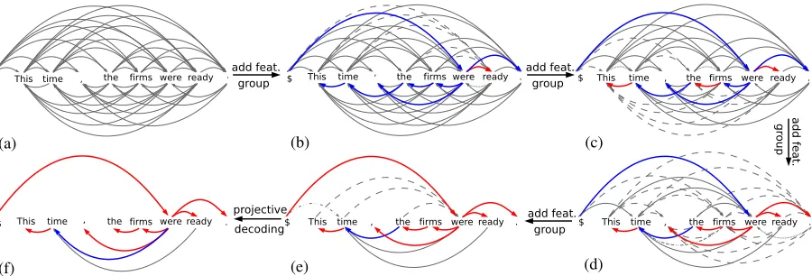
Figure 1: Dynamic feature selection for dependency parsing. (a) Start with all possible edges except those filtered by the length dictionary. (b) – (e) Add the next group of feature templates and parse using the non-projective parser. Predicted trees are shown as blue and red edges, where red indicates the edges that we then decide to lock. Dashed edges are pruned because of having the same child as a locked edge; 2-dot-3-dash edges are pruned because of crossing with a locked edge; fine-dashed edges are pruned because of forming a cycle with a locked edge; and 2-dot-1-dash edges are pruned since the root has already been locked with one child. (f) Final projective parsing.
3.1 Sequential Decision Making
Our work is motivated by recent progress on dy-namic feature selection (Benbouzid et al., 2012; He et al., 2012; Grubb and Bagnell, 2012), where fea-tures are added sequentially to a test instance based on previously acquired features and intermediate prediction results. This requires sequential decision making. Abstractly, when the system is in some state
s ∈ S, it chooses an action a = π(s)from the ac-tion setAusing its policyπ, and transitions to a new
states0, inducing some cost. In the specific case of
dynamic feature selection, when the system is in a given state, it decides whether to add some more features or to stop and make a prediction based on the features added so far. Usually the sequential de-cision making problem is solved by reinforcement learning (Sutton and Barto, 1998) or imitation learn-ing (Abbeel and Ng, 2004; Ratliff et al., 2004).
The dynamic feature selection framework has been successfully applied to supervised classifica-tion and ranking problems (Benbouzid et al., 2012; He et al., 2012; Gao and Koller, 2010). Below, we design a version that avoids overhead in our struc-tured prediction setting. As there are n2 possible
edges on a sentence of lengthn, we wish to avoid
the overhead of making many individual decisions about specific features on specific edges, with each decision considering the current scores of all other edges. Instead we will batch the work of dynamic
feature selection into a smaller number of coarse-grained steps.
3.2 Strategy
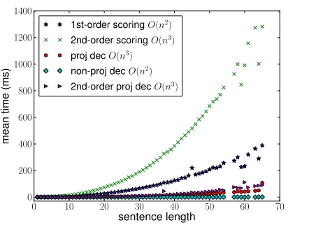
To speed up graph-based dependency parsing, we first investigate time usage in the parsing process on our development set, section 22 of the Penn Treebank (PTB) (Marcus et al., 1993). In Fig-ure 2, we observe that (a) featFig-ure computation took more than 80% of the total time; (b) even though non-projective decoding time grows quadratically in terms of the sentence length, in practice it is al-most negligible compared to the projective decoding time, with an average of 0.23 ms; (c) the second-order projective model is significantly slower due to higher asymptotic complexity in both the scoring and decoding stages.
At each stage of our algorithm, we need to de-cide whether to use additional features to refine the edge scores. As making this decision separately for each of the n2 possible edges is expensive, we
0 10 20 30 40 50 60 70 sentence length
0 200 400 600 800 1000 1200 1400
mean
time
(ms)
1st-order scoringO(n2)
2nd-order scoringO(n3)
proj decO(n3)
non-proj decO(n2)
[image:4.612.76.297.64.225.2]2nd-order proj decO(n3)
Figure 2: Time comparison of scoring time and decoding time on English PTB section 22.
n edges, and we use a classifier to decide which
of these edges are reliable enough that we should “lock” them—i.e., commit to including them in the final tree. This is the only decision that our policy
π must make. Locked (red) edges are definitely in
the final tree. We also do constraint propagation: we rule out all edges that conflict with the locked edges, barring them from appearing in the final tree.3
Con-flicts are defined as violation of the projective pars-ing constraints:
• Each word has exactly one parent • Edges cannot cross each other4 • The directed graph is non-cyclic • Only one word is attached to the root
For example, in Figure 1(d), the dashed edges are removed because they have the same child as one of the locked (red) edges. The 2-dot-3-dash edgetime
← firms is removed because it crosses the locked
edge(comma)←were(whereas we ultimately seek
a projective parse). The fine dashed edge were ←
(period) is removed because it forms a cycle with were → (period). In Figure 1(e), the 2-dot-1-dash
edge (root) → time is removed since we allow the
root to have only one modifier.
3Constraint propagation also automatically locks an edge
when all other edges with the same child have been ruled out.
4A reviewer asks about the cost of finding edges that cross a
locked edge. Naively this isO(n2). But at mostnedges will be
locked during the entire algorithm, for a totalO(n3)runtime—
the same asonecall to projective parsing, and far faster in prac-tice. With cleverness this can even be reduced toO(n2logn).
Once constraint propagation has finished, we visit all edges (gray) whose fate is still unknown, and up-date their scores in parallel by adding the next group of features.
As a result, most edges will be locked in or ruled out without needing to look up all of their features. Some edges may still remain uncertain even after in-cluding all features. If so, a final iteration (Figure 1 (f)) uses the slower projective parser to resolve the status of these maximally uncertain edges. In our example, the parser does not figure out the correct parent oftimeuntil this final step. This final,
accu-rate parser can use its own set of weighted features, including higher-order features, as well as the pro-jectivity constraint. But since it only needs to re-solve the few uncertain edges, both scoring and de-coding are fast.
If we wanted our parser to be able to produce non-projective trees, then we would skip this final step or have it use a higher-order non-projective parser. Also, at earlier steps we would not prune edges crossing the locked edges.
4 Methods
Our goal is to produce a faster dependency parser by reducing the feature computation time. We assume that we are given three increasingly accurate but in-creasingly slow parsers that can be called as sub-routines: a order non-projective parser, a first-order projective parser, and a second-first-order projec-tive parser. In all cases, their feature weights have already been trained using the full set of features,
and we will not change these weights. In general we will return the output of one of the projective parsers. But at early iterations, the non-projective parser helps us rapidly consider interactions among edges that may be relevant to our dynamic decisions.
4.1 Feature Template Ranking
in-0 50 100 150 200 250 300 350 400 Number of feature templates used
0.5 0.6 0.7 0.8 0.9
Unlabeled
attachment
score
(U
AS)
[image:5.612.79.297.66.226.2]1st-order non-proj 1st-order proj 2nd-order
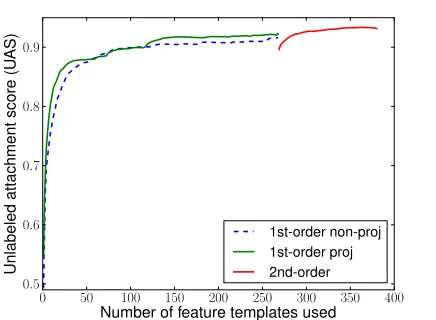
Figure 3: Forward feature selection result using the non-projective model on English PTB section 22.
stead select the feature template with the highest ra-tio of accuracy improvement to runtime. However, for simplicity we do not consider this: after group-ing (see below), minor changes of the ranks within a group have no effect. The accuracy is evaluated by running the first-order non-projective parser, since we will use it to make most of the decisions. The 112 second-order feature templates are then ranked by adding them in a similar greedy fashion (given that all first-order features have already been added), evaluating with the second-order projective parser.
We then divide this ordered list of feature tem-plates intoKgroups: {T1, T2, . . . , TK}. Our parser adds an entire group of feature templates at each step, since adding one template at a time would re-quire too many decisions and obviate speedups. The simplest grouping method would be to put an equal number of feature templates in each group. From Figure 3 we can see that the accuracy increases sig-nificantly with the first few templates and gradually levels off as we add less valuable templates. Thus, a more cost-efficient method is to split the ranked list into several groups so that the accuracy increases by roughly the same amount after each group is added. In this case, earlier stages are fast because they tend to have many fewer feature templates than later stages. For example, for English, we use 7 groups of first-order feature templates and 4 groups of second-order feature templates. The sequence of group sizes is 1, 4, 10, 12, 47, 33, 161 and 35, 29, 31, 17 for first- and second-order parsing respectively.
4.2 Sequential Feature Selection
Similar to the length dictionary filter of Rush and Petrov (2012), for each test sentence, we first de-terministically remove edges longer than the maxi-mum length of edges in the training set that have the same head POS tag, modifier POS tag, and direction. This simple step prunes around40%of the non-gold edges in our Penn Treebank development set (Sec-tion 6.1) at a cost of less than0.1%in accuracy.
Given a test sentence of length n, we start with
a complete directed graph G(V,E), where E = {hh, mi: h ∈ [0, n], m ∈ [1, n]}. After the length dictionary pruning step, we computeT1 for all re-maining edges to obtain a pruned weighted directed graph. We predict a parse tree using the features so far (other features are treated as absent, with value 0). Then for each edge in this intermediate tree, we use a binary linear classifier to choose between two actions: A = {lock,add}. The lockaction ensures
thathh, mi appears in the final parse tree by prun-ing edges that conflict withhh, mi.5 If the classi-fier is not confident enough about the parent of m,
it decides to add to gather more information. The addaction computes the next group of features for
hh, miand all other competing edges with childm.
(Since we classify the edges one at a time, deci-sions on one edge may affect later edges. To im-prove efficiency and reduce cascaded error, we sort the edges in the predicted tree and process them as above in descending order of their scores.)
Now we can continue with the second iteration of parsing. Overall, our method runs up toK =K1+
K2 iterations on a given sentence, where we have
K1 groups of first-order features andK2 groups of second-order features. We run K1 −1 iterations of non-projective first-order parsing (adding groups
T1, . . . , TK1−1), then 1 iteration of projective first-order parsing (adding groupTK1), and finallyK2 it-erations of projective second-order parsing (adding groupsTK1+1, . . . TK).
Before each iteration, we use the result of the pre-vious iteration (as explained above) to prune some edges and add a new group of features to the rest. We
5If the conflicting edge is in the current predicted parse tree
then run the relevant parser. Each of the three parsers has a different set of feature weights, so when we switch parsers on roundsK1 andK1 + 1, we must alsochangethe weights of the previously added
fea-tures to those specified by the new parsing model. In practice, we can stop as soon as the fate of all edges is known. Also, if no projective parse tree can be constructed at roundK1 using the available unpruned edges, then we immediately fall back to returning the non-projective parse tree from round
K1−1. This FAIL case rarely occurs in our experi-ments (fewer than 1% of sentences).
We report results both for a first-order system whereK2 = 0(shown in Figure 1 and Algorithm 1) and for a second-order system whereK2 >0.
Algorithm 1DynFS(G(V,E),π)
E ← {hh, mi: |h−m| ≤lenDict(h, m)} AddT1to all edges inE
ˆ
y←non-projective decoding
fori= 2toK do
Esort ←sort unlocked edges{E : E ∈ yˆ}in descending order of their scores
forhh, mi ∈ Esortdo
ifπ(ψ(hh, mi)) ==lockthen
E ← E \ {{hh0, mi ∈ E: h0 6=h}S {hh0, m0i ∈ E: crosseshh, mi}S {hh0, m0i ∈ E: cycle withhh, mi}}
ifh== 0then
E ← E \ {h0, m0i ∈ E:m06=m}
end if else
AddTi to{hh0, m0i ∈ E: m0==m} end if
end for
ifi==K then
ˆ
y←projective decoding
else ifi6=KorFAILthen
ˆ
y←non-projective decoding
end if end for returnyˆ
5 Policy Training
We cast this problem as an imitation learning task and use Dataset Aggregation (DAgger) Ross et al. (2011) to train the policy iteratively.
5.1 Imitation Learning
In imitation learning (also called apprenticeship learning) (Abbeel and Ng, 2004; Ratliff et al., 2004), instead of exploring the environment directed by its feedback (reward) as in typical reinforcement learn-ing problems, the learner observes expert demon-strations and aims to mimic the expert’s behavior. The expert demonstration can be represented as tra-jectories of state-action pairs, {(st, at)} where tis the time step. A typical approach to imitation learn-ing is to collect supervised data from the expert’s trajectories to learn a policy (multiclass classifier), where the input isψ(s), a feature representation of the current state (we call these policy features to
avoid confusion with theparsing features), and the
output is the predicted action (label) for that state. In the sequential feature selection framework, it is hard to directly apply standard reinforcement learn-ing algorithms, as we cannot assign credit to certain features until the policy decides to stop and let us evaluate the prediction result. On the other hand, knowing the gold parse tree makes it easy to ob-tain expert demonstrations, which enables imitation learning.
5.2 DAgger
Since the above approach collects training data only from the expert’s trajectories, it ignores the fact that the distribution of states at training time and that at test time are different. If the learned policy can-not mimic the expert perfectly, one wrong step may lead to states never visited by the expert due to cu-mulative errors. This problem of insufficient explo-ration can be alleviated by iteratively learning a pol-icy trained under states visited by both the expert and the learner (Ross et al., 2011; Daum´e III et al., 2009; K¨a¨ari¨ainen, 2006).
Ross et al. (2011) proposed to train the policy iter-atively and aggregate data collected from the previ-ous learned policy. Letπ∗denote the expert’s policy
andsπi denote states visited by executingπi. In its
simplest parameter-free form, in each iteration, we first run the most recently learned policyπi; then for each statesπion the trajectory, we collect a training
example(ψ(sπi), π
∗(s
πi))by labeling the state with
expert’s trajectory. Thus we can obtain a policy that performs well under its own induced state distribu-tion.
5.3 DAgger for Feature Selection
In our case, the expert’s decision is rather straight-forward. Replace the policy π in Algorithm 1 by
an expert. If the edge under consideration is a gold edge, it executes lock; otherwise, it executes add.
Basically the expert “cheats” by knowing the true tree and always making the right decision. On our PTB dev set, it can get96.47%accuracy6 with only 2.9% of the first-order features. This is an upper bound on our performance.
We present the training procedure in Algorithm 2. We begin by partitioning the training set into
N folds. To simulate parsing results at test time,
when collecting examples on Ti, similar to cross-validation, we use parsers trained onT¯i = T \ Ti. Also note that we show only one pass over training sentences in Algorithm 2; however, multiple passes are possible in practice, especially when the training data is limited.
Algorithm 2DAgger(T,π∗)
Split the training sentences T into N folds
T1,T2, . . . ,TN
InitializeD ← ∅,π1←π∗
fori= 1toN do forG(V,E)∈ Tido
Sample trajectories {(sπi, πi(sπi))} by
DynFS(G(V,E), πi)
D ← D S
{(ψ(s), π∗(s)}
end for end for
Train policyπi+1onD
returnBestπievaluated on development set
5.4 Policy Features
Our linear edge classifier uses a feature vectorψthat
concatenates all previously acquired parsing fea-tures together with “meta-feafea-tures” that reflect con-fidence in the edge. The classifier’s weights are fixed
6The imperfect performance is because the accuracy is
mea-sured with respect to the gold parse trees. The expert only makes optimal pruning decisions but the performance depends on the pre-trained parser as well.
across iterations, butψ(edge) changes per iteration.
We standardize the edge scores by a sigmoid func-tion. Let s˙ denote the normalized score, defined bys˙θ(hh, mi) = 1/(1 + exp{−sθ(hh, mi)}). Our
meta-features forhh, miinclude
• current normalized score, and normalized score before adding the current feature group • margin to the highest scoring competing edges,
i.e., s˙(w,hh, mi)−maxh0s˙(w,hh0, mi)
whereh0 ∈[0, n]andh0 6=h
• index of the next feature group to be added
We also tried more complex meta-features, for ex-ample, mean and variance of the scores of compet-ing edges, and structured features such as whether the head ofeis locked and how many locked
chil-dren it currently has. It turns out thatgiven all the parsing features, the margin is the most
discrimi-native feature. When it is present, other meta-features we added do not help much, Thus we do not include them in our experiments due to overhead.
6 Experiment
6.1 Setup
We generate dependency structures from the PTB constituency trees using the head rules of Yamada and Matsumoto (2003). Following convention, we use sections 02–21 for training, section 22 for de-velopment and section 23 for testing. We also re-port results on six languages from the CoNLL-X shared task (Buchholz and Marsi, 2006) as sug-gested in (Rush and Petrov, 2012), which cover a variety of language families. We follow the stan-dard training/test split specified in the CoNLL-X data and tune parameters by cross validation when training the classifiers (policies). The PTB test data is tagged by a Stanford part-of-speech (POS) tagger (Toutanova et al., 2003) trained on sections 02–21. We use the provided gold POS tags for the CoNLL test data. All results are evaluated by the unlabeled attachment score (UAS). For fair comparison with previous work, punctuation is included when com-puting parsing accuracy of all CoNLL-X languages but not English (PTB).
se-Language Method First-order Second-order
Speedup Cost(%) UAS(D) UAS(F) Speedup Cost(%) UAS(D) UAS(F)
Bulgarian DYNFS 3.44 34.6 91.1 91.3 4.73 16.3 91.6 92.0
VINEP 3.25 - 90.5 90.7 7.91 - 91.6 92.0
Chinese DYNFS 2.12 42.7 91.0 91.3 2.36 31.6 91.6 91.9
VINEP 1.02 - 89.3 89.5 2.03 - 90.3 90.5
English DYNFS 5.58 24.8 91.7 91.9 5.27 49.1 92.5 92.7
VINEP 5.23 - 91.0 91.2 11.88 - 92.2 92.4
German DYNFS 4.71 21.0 89.2 89.3 6.02 36.6 89.7 89.9
VINEP 3.37 - 89.0 89.2 7.38 - 90.1 90.3
Japanese DYNFS 4.80 15.6 93.7 93.6 8.49 7.53 93.9 93.9
VINEP 4.60 - 91.7 92.0 14.90 - 92.1 92.0
Portuguese DYNFS 4.36 32.9 87.3 87.1 6.84 40.4 88.0 88.2
VINEP 4.47 - 90.0 90.1 12.32 - 90.9 91.2
Swedish DYNFS 3.60 37.8 88.8 89.0 5.04 22.1 89.5 89.8
[image:8.612.71.547.57.254.2]VINEP 4.64 - 88.3 88.5 13.89 - 89.4 89.7
Table 1: Comparison of speedup and accuracy with the vine pruning cascade approach for six languages. In the setup,
DYNFS means our dynamic feature selection model, VINEP means the vine pruning cascade model, UAS(D) and
UAS(F) refer to the unlabeled attachment score of the dynamic model (D) and the full-feature model (F) respectively. For each language, the speedup is relative to its corresponding first- or second-order model using the full set of features. Results for the vine pruning cascade model are taken from Rush and Petrov (2012). The cost is the percentage of feature templates used per sentence on edges that arenot pruned by the dictionary filter.
lect the best policy evaluated on the development set among the 20 policies obtained from each iteration.
6.2 Baseline Models
We use the publicly available implementation of MSTParser7(with modifications to the feature
com-putation) and its default settings, so the feature weights of the projective and non-projective parsers are trained by the MIRA algorithm (Crammer and Singer, 2003; Crammer et al., 2006).
Our feature set contains most features proposed in the literature (McDonald et al., 2005a; Koo and Collins, 2010). The basic feature components in-clude lexical features (token, prefix, suffix), POS features (coarse and fine), edge length and direction. The feature templates consists of different conjunc-tions of these components. Other than features on the head word and the child word, we include fea-tures on in-between words and surrounding words as well. For PTB, our first-order model has 268 feature templates and 76,287,848 features; the second-order model has 380 feature templates and 95,796,140 fea-tures. The accuracy of our full-feature models is
7
http://www.seas.upenn.edu/˜strctlrn/ MSTParser/MSTParser.html
comparable or superior to previous results.
6.3 Results
0 1 2 3 4 5 6
Feature selection stage 0.0
0.2 0.4 0.6 0.8 1.0
Time/Accur
acy/Edge
Percentage runtime %
UAS % remaining edge % locked edge % pruned edge %
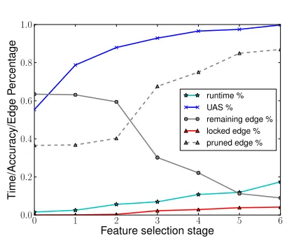
Figure 4: System dynamics on English PTB section 23. Time and accuracy are relative to those of the baseline model using full features. Red (locked), gray (unde-cided), dashed gray (pruned) lines correspond to edges shown in Figure 1.
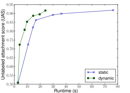
[image:8.612.317.537.410.580.2]0 10 20 30 40 50 60 70 80 Runtime (s)
0.50 0.55 0.60 0.65 0.70 0.75 0.80 0.85 0.90 0.95
Unlabeled
attachment
score
(U
AS)
[image:9.612.76.297.57.216.2]static dynamic
Figure 5: Pareto curves for the dynamic and static ap-proaches on English PTB section 23.
parsing. Thespeedupfor each language is defined as
the speed relative to its full-feature baseline model. We take results reported by Rush and Petrov (2012) for the vine pruning model. As speed comparison for parsing largely relies on implementation, we also report the percentage of feature templates chosen for each sentence. Thecostcolumn shows the average
number of feature templates computed for each sen-tence, expressed as a percentage of the number of feature templates if we had only pruned using the length dictionary filter.
From the table we notice that our first-order model’s performance is comparable or superior to the vine pruning model, both in terms of speedup and accuracy. In some cases, the model with fewer features even achieves higher accuracy than the model with full features. The second-order model, however, does not work as well. In our experi-ments, the second-order model is more sensitive to false negatives, i.e. pruning of gold edges, due to larger error propagation than the first-order model. Therefore, to maintain parsing accuracy, the policy must make high-precision pruning decisions and be-comes conservative. We could mitigate this by train-ing the original parstrain-ing feature weights in conjunc-tion with our policy feature weights. In addiconjunc-tion, there is larger overhead during when checking non-projective edges and cycles.
We demonstrate the dynamics of our system in Figure 4 on PTB section 23. We show how the run-time, accuracy, number of locked edges and unde-cided edges change over the iterations in our
first-order dynamic projective parsing. From iterations 1 to 6, we obtain parsing results from the non-projective parser; in iteration 7, we run the non-projective parser. The plot shows relative numbers (percent-age) to the baseline model with full features. The number of remaining edges drops quickly after the second iteration. From Figure 3, however, we notice that even with the first feature group which only con-tains one feature template, the non-projective parser can almost achieve50%accuracy. Thus, ideally, our policy should have locked that many edges after the first iteration. The learned policy does not imitate the expert perfectly, either because our policy fea-tures are not discriminative enough, or because a lin-ear classifier is not powerful enough for this task.
Finally, to show the advantage of making dynamic decisions that consider the interaction among edges on the given input sentence, we compare our results with a static feature selection approach on PTB sec-tion 23. The static algorithm does no pruning except by the length dictionary at the start. In each iteration, instead of running a fast parser and making deci-sions online, it simply adds the next group of feature templates to all edges. By forcing both algorithms to stop after each stage, we get the Pareto curves shown in Figure 5. For a given level of high accu-racy, our dynamic approach (black) is much faster than its static counterpart (blue).
7 Conclusion
In this paper we present a dynamic feature selec-tion algorithm for graph-based dependency parsing. We show that choosing feature templates adaptively for each edge in the dependency graph greatly re-duces feature computation time and in some cases improves parsing accuracy. Our model also makes it practical to use an even larger feature set, since features are computed only when needed. In future, we are interested in training parsers favoring the dy-namic feature selection setting, for example, parsers that are robust to missing features, or parsers opti-mized for different stages.
Acknowledgements
References
P. Abbeel and A. Y. Ng. 2004. Apprenticeship learning via inverse reinforcement learning. InProceedings of ICML.
D. Benbouzid, R. Busa-Fekete, and B. K´egl. 2012. Fast classification using space decision DAGs. In Proceed-ings of ICML.
S. Bergsma and C. Cherry. 2010. Fast and accurate arc filtering for dependency parsing. In Proceedings of COLING.
S. Buchholz and E. Marsi. 2006. CoNLL-X shared task on multilingual dependency parsing. InCoNLL.
Xavier Carreras. 2007. Experiments with a higher-order projective dependency parser. InProceedings of the CoNLL Shared Task Session of EMNLP-CoNLL.
Eugene Charniak, Mark Johnson, Micha Elsner, Joseph Austerweil, David Ellis, Isaac Haxton, Catherine Hill, R. Shrivaths, Jeremy Moore, Michael Pozar, and Theresa Vu. 2006. Multilevel coarse-to-fine PCFG parsing. InProceedings of ACL.
Y. J. Chu and T. H. Liu. 1965. On the shortest arbores-cence of a directed graph. Science Sinica, 14.
Koby Crammer and Yoram Singer. 2003. Ultraconserva-tive online algorithms for multiclass problems. Jour-nal of Machine Learning Research, 3:951–991.
Koby Crammer, Ofer Dekel, Joseph Keshet, Shai Shalev-Shwartz, and Yoram Singer. 2006. Online passive-aggressive algorithms. Journal of Machine Learning Research, 7:551–585.
Hal Daum´e III, John Langford, and Daniel Marcu. 2009. Search-based structured prediction. Machine Learn-ing Journal (MLJ).
J. Edmonds. 1967. Optimum branchings. Journal
of Research of the National Bureau of Standards,
(71B):233–240.
Jason Eisner. 1996. Three new probabilistic models for dependency parsing: an exploration. InProceedings of COLING.
Rong-En Fan, Kai-Wei Chang, Cho-Jui Hsieh, Xiang-Rui Wang, and Chih-Jen Lin. 2008. LIBLINEAR: A li-brary for large linear classification. Journal of Ma-chine Learning Research, 9:1871–1874.
Tianshi Gao and Daphne Koller. 2010. Active classifi-cation based on value of classifier. InProceedings of NIPS.
Alexander Grubb and J. Andrew Bagnell. 2012.
SpeedBoost: Anytime prediction with uniform near-optimality. InAISTATS.
He He, Hal Daum´e III, and Jason Eisner. 2012. Cost-sensitive dynamic feature selection. InICML Infern-ing Workshop.
Matti K¨a¨ari¨ainen. 2006. Lower bounds for
reduc-tions. Talk at the Atomic Learning Workshop (TTI-C), March.
Terry Koo and Michael Collins. 2010. Efficient third-order dependency parsers. InProceedings of ACL.
Mitchell P. Marcus, Beatrice Santorini, and Mary Ann Marcinkiewicz. 1993. Building a large annotated
cor-pus of English: The Penn Treebank. Computational
Linguistics, 19(2):313–330.
Andr´e F. T. Martins, Dipanjan Das, Noah A. Smith, and Eric P. Xing. 2008. Stacking dependency parsers. In
Proceedings of EMNLP.
Ryan McDonald and Fernando Pereira. 2006. On-line learning of approximate dependency parsing al-gorithms. InProceedings of EACL, pages 81–88.
Ryan McDonald, K. Crammer, and Fernando Pereira. 2005a. Online large-margin training of dependency parsers. InProceedings of ACL.
Ryan McDonald, Fernando Pereira, Kiril Ribarov, and Jan Hajiˇc. 2005b. Non-projective dependency parsing using spanning tree algorithms. InProc. of EMNLP.
N. Ratliff, D. Bradley, J. A. Bagnell, and J. Chestnutt. 2004. Boosting structured prediction for imitation learning. InProceedings of ICML.
B. Roark and K. Hollingshead. 2008. Classifying chart cells for quadratic complexity context-free inference. InProceedings of COLING.
St´ephane. Ross, Geoffrey J. Gordon, and J. Andrew. Bag-nell. 2011. A reduction of imitation learning and structured prediction to no-regret online learning. In
Proceedings of AISTATS.
Alexander Rush and Slav Petrov. 2012. Vine pruning for efficient multi-pass dependency parsing. In Proceed-ings of NAACL.
David A. Smith and Jason Eisner. 2008. Dependency parsing by belief propagation. InEMNLP.
Richard S. Sutton and Andrew G. Barto. 1998.
Rein-forcement Learning : An Introduction. MIT Press.
R. E. Tarjan. 1977. Finding optimum branchings. Net-works, 7(1):25–35.
Kristina Toutanova, Dan Klein, Christopher Manning, and Yoram Singer. 2003. Feature-rich part-of-speech tagging with a cyclic dependency network. InNAACL.
Paul Viola and Michael Jones. 2004. Robust feal-time face detection. International Journal of Computer Vi-sion, 57:137–154.
Qin Iris Wang, Dekang Lin, and Dale Schuurmans. 2007. Simple training of dependency parsers via structured boosting. InProceedings of IJCAI.
David Weiss and Ben Taskar. 2010. Structured predic-tion cascades. InProceedings of AISTATS.