Online Full Text

Abstract—Dynamic programming partitions the problem into not completely independent sub problems and solves every sub problem just once and then saves its answer in a table in forward path. The required space for this table usually is proportional to the square of the input size that is contained a huge part of memory. In this paper we describe a new method for reducing the space complexity of dynamic programming. In this method, that information is saved in forward path, which they cannot reproduce at backward path. A stack is used for saving this data. By this way the path of constructing optimal solution can be reproduced by using saved information in stack. We can find some rules for selecting saved information. As an example we applied this method on Longest Common Subsequence (LCS) problem for global alignment of DNA sequences. As we examined in proposed algorithm, the size of stack in comparing to using space for LCS algorithm was reduced about 10 times and we could increase the input size in global alignment

Index Terms—bidirectional method, global alignment, Longest Common Subsequence (LCS).

I. INTRODUCTION

Dynamic programming is typically applied to optimization problems and partitions the problem into not completely independent sub problems. A dynamic-programming algorithm solves every sub problem just once and then saves its answer in a table, thereby avoiding the work of recomputing the answer every time the sub problem is encountered.

The development of a dynamic-programming algorithm can be broken into a sequence of four steps [1]:

1) Characterize the structure of an optimal solution. 2) Recursively defines the value of an optimal solution. 3) Compute the value of an optimal solution in a bottom-up

fashion (forward step).

4) 4. Construct an optimal solution from computed information (backward step).

Steps 1–3 form the basis of a dynamic-programming solution to a problem. Step 4 can be omitted if only the value of an optimal solution is required. When we do perform step 4, we sometimes maintain additional information during the

R.Khayami is with the Departement of Computer Engineering, Islamic Azad University of Shiraz, Iran (corresponding author), phone: 0098-917-100-4856; fax: 0098-711-6271747;

(e-mail: [email protected]).

E. Parvinnia, Departement of Computer Science and Engineering, Shiraz University, Shiraz, Iran (e-mail: [email protected]).

computation in step 3 in a table. This table traverses inversely in step 4 to construct an optimal solution. The required space for this table usually is proportional to the square of the input size that is contained a huge part of memory. Therefore, in some problems with large input size, the space of memory is too big that we cannot run the program. As an example, we can point to Longest Common Subsequence (LCS) algorithm.

The LCS problem is one of the classical and well-studied problems in computer science which has extensive applications in diverse areas ranging from spelling error corrections to molecular biology. The LCS problem is a common task in DNA sequence analysis, and has applications to genetics and molecular biology [2]-[5]. The classic dynamic programming solution to LCS problem, invented by Wagner and Fischer [6], has O(n2) worst case running time. However, several algorithms exist with complexities depending on other parameters. For a comprehensive comparison of the well-known algorithms for LCS problem and study of their behavior in various application environments the readers are referred to [7]. LCS is the only algorithm that has optimal solution and independent to the shape of its inputs. Because of the space complexity of this algorithm is the multiplication of sequences’ lengths; we cannot use it for long sequences. For example for two sequences with 50 Kb lengths, we need at least 2.5 GB memory. Therefore we cannot use LCS for long sequences on ordinary computers.

This large space is used for saving forward path in step 3 to construct longest common subsequence in step 4. If it is possible to produce the information in forward step at backward path, it is possible not to save all the table of forward path. By this way, the used memory is reduced but this is sometimes impossible and we need some information that without them, we cannot reproduce primary path.

This article proposes a solution that with using it we can reduce memory complexity in dynamic programming at forward path. In this method, that information is saved which they cannot reproduce at backward path. A stack is used for saving this information. By this way the path of constructing optimal solution can be reproduced by using saved information in stack at step 4. This method was applied on LCS algorithm with DNA sequences as input. Because of reducing memory space, the input sequences could be increased up to several times proportion to LCS algorithm. The rest of the paper is organized as follows. In Section 2, we present all the definitions and notations to introduce the

A Novel Stack based Dynamic Programming for

Reducing Memory Complexity

Applied on DNA Sequences

concepts of LCS which we wish to handle in this paper. Also, we review the traditional dynamic programming techniques to solve the global alignment problem. In Sections 3, we present new algorithm for all the variants discussed in this paper. In particular, we first present reproduction rules implement-able in dynamically finding LCS and then explain preprocessing to find the variables not needed in backward iteration. In section 4, some experimental result is described and finally we have a conclusion and propose some future works.

II. 2. RELATED WORKS

The comparison of biological sequences is one of the oldest problems in computational biology, and early work on the problem resulted in what were arguably the first highly successful and widely adopted applications of computer science to biology. It became apparent early on that alignment programs could be divided into two types: first. Local alignment methods (Smith and Waterman, 1981; Gotoh, 1982; Pearson and Lipman, 1988; Altschul et al., 1990; Huang and Miller, 1991; Burkhardt et al., 1999; Arslan et al., 2001; Ma et al., 2002) are designed to search for highly similar regions in two sequences, where the regions of similarity are not necessarily conserved in order and orientation. Local alignment algorithms are generally very useful in finding similarity between regions that may be related but are inverted or rearranged with respect to each other. A problem with local alignment algorithms is that, because of the weaker assumptions in place, there is less power in finding weakly conserved regions; furthermore, identified conserved regions may not be true homolog's (i.e., related via a common ancestor). Global alignment algorithms (e.g., Needleman and Wunsch 1970) are suitable when an extra assumption holds, namely, that the highly similar regions in the sequences appear in the same order and orientation. Global alignment algorithms have been found to be useful in many situations because biological sequences from related organisms tend to satisfy the order assumption. Because we must examine genome appear to have order and orientation preserved with long length (up to 8 Mb for human), the global alignment models lead to slow algorithms that are also very memory intensive[8],[9].

There are 3 optimal solutions for global alignment problem. The first is LCS algorithm that is based on dynamic programming and has time and memory complexity O(M*N). M and N are the length of two sequences. It is completely described in next subsection.

The second is bidirectional algorithm that is based on LCS. This method has two parts. In part one, forward step of LCS is done and for reducing memory, only current and right previous row of table is saved. Then after finishing forward path, we have only the last row and the row before it. In part two, backward step of LCS is done by saving information in the last two rows. Everywhere the information is not enough to construct backward path, part one of algorithm is run to find that information. When two paths received each other, we have a point that divides each sequence to two sections. After that the algorithm can be applied on section 1 and section 2 of each sequence individually and repeatedly.

Part 1 of bidirectional method has O(M*N) time complexity and O(2*min(M,N)) memory complexity. In part 2, part 1 is called and this is continued repeatedly. Therefore, although memory complexity is reduced, final time complexity is larger than LCS algorithm [10].

The third is based on LCS algorithm, too. It is a divide and conquers approach that performs alignment in linear space complexity for the expense of just doubling the computational time. The algorithm is described in next subsection).

A. Longest Common Subsequence Algorithm (LCS) Definition 1: An initial substring S' of a string S is a sequence of characters S'[i] = S[i] for i = 1, …, u where u is length of S' and is less than or equal to length of S.

The Whole of process can be saved in two (M+1) x (N+1) tables, named TblValues and TblParents, such that M and N are the length of SL as longer string and Ss as smaller one respectively. Rows are indexed by 0… M and Columns are indexed by 0… N.

TblValues[i][j] represents a value which indicates the length of the longest common sequence between two substrings SLi and SSj . SLi is an initial substring of SL where its length is equal to i. Also SSj is, in a same way, an initial substring of SS where its length is equal to j.

This process is done in two iterations, forward and backward.

In the forward iteration, elements of matrices TblValues and TblParents, as described in following, are filled by a dynamic approach. Assume that the first character of each string is located at index 1. Hence, for every i and j, TblValues[i][0]=TblValues[0][j]=0.Then, for every i, j >0

(1)

TblParents[i][j] also indicates, in which way TblValues[i][j] is made based on (1).TblValues[M][N] indicates the length of LCS (Longest Common Sequence) but a backward iteration is needed to produce the LCS itself by using the matrix TblParents. Values which can be assigned to elements of TblParents are [\ , ←, ↑] in order of their priorities. If TblParents[i][j] is ← , the value of the associates element in TblValues is equal to its left neighbor element i.e., TblValues [i] [j-1]. In this case, LCS of SLi and SSj, as the current state, can be equal to LCS of SLi and SSj-1, as the parent state. In this case, we call the left neighbor element as the parent of current element. In the same way, ↑ indicates the top neighbor element as the parent such that LCS of current state is the same as LCS of SLi-1 and SSj, as the parent state. If SL[i] is equal to SS[j], TblParents[i] [j] is set to'\' in order o identify the top-left neighbor as the parent. This is the only case, in which the length of current LCS is one more than the length of LCS of parent state. If more than one value can be chosen to assign, the one with more priority is selected.

In backward iteration, we start from the element in row M and column N, as the end state. The process goes on by considering parent of current state as the new current state in

(

)

⎪ ⎩ ⎪ ⎨ ⎧

− −

= +

− − =

otherwise j

i TBlV j i TblV

j S S i L S if j i TblV j i TblV

] 1 ][ [ ], ][ 1 [ max

each level until it reaches to the element in row and/or column 0. From now the path which connects these states in this order is named optimal sequence, in this article. Any visited state which is valued \ identifies its associated character in SL or SS (which are the same) as a character of LCS of SL and SS. We cannot reproduce the TblParents elements in backward iteration. Therefore, if the characters of LCS are desired, at least matrix TblParents must be saved in forward iteration. Although the TblValues is not necessary saved with M rows, Saving TblParents takes O(M*N) memory.

There is a procedure to reproduce the ith row of TblParents by using ith row of TblValues, as shown in (2):

⎪ ⎩ ⎪ ⎨ ⎧

↑

− =

←

= =

otherwise

j i TblV j i TblV elseif

j S i S if j i TblP

S L

] 1 ][ [ ] ][ [

] [ ] [ \ ] ][

[ (2)

But this procedure cannot be used to reproduce the whole of rows of TblParents unless TblValues is saved completely or it can be reproduced independent of TblParents. Saving TblValues takes O (M.N) memory as same as TblParents[11]-[13].

B. Divide and Conqure Aalgorithm

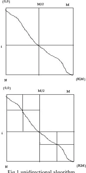
The longest path in the TblParents passes through an unknown middle point (i , M/2). For simplicity assume M is even. Let's try to find middle point instead of trying to find the entire longest path. This can be done in linear space by computing the lengths of the longest path from (0,0) to (i,M/2) for 0≤ i ≤N and the length of longest path from (i,M/2) to (N,M) reversly. The value L = TblValues[i][M/2] + reversed(Tblvalues[i][M/2]) is the length of the longest path from (0,0) to (N,M) passing through the point (i,M/2). Therefore, with maximizing L, the length of longest path is computed and a middle point is identified.

Computing these values required the time equal to area of the left rectangle from column 1 to m/2 plus the area of the right rectangle from column M/2 +1 to M and the space O(N) Fig. 1. After the middle point (i,M/2) is found,the problem of finding the logest path from (0,0)to (N,M) can be portioned into two subproblems: finding the longest path from (0,0) to middle point (i,M/2) and finding the longest path from middle point to (N,M). instead of trying to find these pathes, we first try to find the middle point in the corresponding rectangles. This can be done in the time equal to the area of these rectangles, which is two times smaller than the area of the original rectangle. Computing in this way, we will find the middle vertices of all rectangles in time area + area/2 + area/4 + … ≤ 2*area and therefore compute the longest path in time O(N*M) and space O(N) [10].

III. PROPOSED ALGORITHM

There are so many dynamic algorithms (commonly graph-based) that should have a backward procedure and use a huge amount of memory to determine the optimal path. In some of them, a state needs the information of all previous states to gain values of its variables. In some others, states are divided into some layers and each state only needs the states

in previous layer. Hence, the memory can be used only to save previous and current layers of states to calculate the optimal

Fig.1 unidirectional algorithm

value. But finding the optimal path needs a backward iteration whereas values of variables in only two last layers are in hand. In case of these algorithms, there is no method to reproduce the unsaved information while the backward procedure is taking place unless it starts again from the start state that is much time consuming. In this case, to reduce the required space, some methods have been proposed such as bidirectional/unidirectional divide and conquer [10]. There is usually no way to reproduce unsaved information of a special state with respect to the information of states which are visited later. But some of these algorithms, such as finding LCS, can reproduce much of this information by a reverse action with respect to the later states which are visited earlier in backward procedure. Hence, the required memory space may decrease to size of two layers even if the optimal path is desired.

reproduced, they will be stacked.

There are some variables in search algorithms which may never be used in backward procedure. These variables are problem dependent and it is not possible to predefine them. Hence with respect to the problem (in this case, regarding the strings) these variables can be specified by a preprocessing in order to reduce both of memory storage and processing time. In fallowing, some preprocessing has been proposed for finding LCS.

Despite, using a stack to save only not reproducible variables reduces the needed memory space but the size of the stack is also so large to be stored in most of high size problems. To overcome this lack, two general methods and one specific method for LCS problem are proposed.

In LCS, the variables are stack in order of row visiting (top to down) and then right to left. Hence, the element at the top of stack is one of not reproducible variables which located in row with bigger index than others and, in having same row index, it is located in the most left position. In this article, some type of storing the stack is considered such that at each level, the element in the lowest row in a specified column which is not yet pop is reachable in O(1). Each element is stored by its value, column number, TRow number and the index of previous element in the stack with the same column number. Also an array, named 'ColumnView', is used to save the index of the last pushed element in the stack with a specified column number. TRow number associated to an element is the minimum row number of elements with the same value and same column. It can also be stored in an array (with the same size as a row) for elements of current row in forward iteration and it may changes in overwriting procedure.

A. Reproduction rules implement-able in dynamically finding LCS:

To reproduce elements of a row from the values exposed by the next row, elements are considered from left to right and their values are calculated by following rules in order of their presentation:

1) If this variable has been stacked (as the top of the stack), it will be pop. Its value is assigned to associated element in matrix, and its reference to the previous element in stack with the same column is utilized to update the array ColumnView.

2) Regarding the next row in TblParents (Which is reproduced by associated row in TblValues) this element is parent of any element, named child, its value can be calculated by the value of child.

3) If values of the bottom neighbor B and bottom right neighbor BR are not similar, BR is certainly one more than B and value of the element in the hand is equal to B. 4) If value of the left neighbor is same as B, value of current

element is B too.

5) If you reach this state, the neighbors in TblValues are valued as shown in Fig. 2 :

B-1 * ? ? B B Fig. 2 reproduction rule5

Where, the '*' identifies the current element at the hand and '?' shows the undetermined value. * can be only B or B-1. Set R and C as the row and column numbers of current element respectively. If the value of element referenced by ColumnView[C] is equal to B, * is located between two elements in column C with value B; hence * is equal to B too. 6) If value of element which is referenced by

ColumnView[C+1] is equal to B, name its TRow number as T. Hence TblValues[T][C+1] is equal to B but surly TblValues[T-1][C+1] is B-1. Hence the parent of element in row T and column C+1 can never be its top neighbor. If SL[T]≠SS[C+1], parent of element in row T and column C+1 is certainly its left neighbor. Hence, TblValues[T][C] is also equal to B. Since T is lower than or equal to R, * is also B.

7) Assume that Y<=R is specified such that for every i between Y and R inclusively, TblValues[i][C-1] is equal to B-1, as shown in Fig. 3:

Y B-1 ? ?

… B-1 ? ?

J B-1 # ?

… B-1 ? ?

R B-1 * ?

R+1 ? B B

C-1 C C+1

Fig. 3 reproduction rule7

Y is a variable which specifies a row index such that TblValues[Y][C-1]is the same as TblValues[R][C-1] but Y is tried to be as minimum as possible. In our implementation, Y is equal to R at the start of reproducing row indexed by R. When value of element located in row R and column C is determined, then Y is updated by (3) to be used for next element.

⎪ ⎩ ⎪ ⎨ ⎧

−

− =

=

otherwise C

R t Grandparen

C R TblV C R TblV elseif Y

Exists C E if C E of TRow Ynew old

1 ) , (

] 1 ][ [ ] ][ [

) ( ) (

(3)

Where, E(R, C) is the element which were or still is referenced by ColumnView[C] such that value of that stacked element is equal to TblValues[R][C]; E(R, C) is also saved in an array for current row and is updated whenever an element is pop from stack. Grandparent (R, C) is presented by (4):

]] [ ][ [ )

,

(RC Appearances R S C t

Grandparen = S (4) Hence, examination of this condition is done in O(1) time complexity and O(k.M) memory complexity.

8) In state that none of above conditions is satisfied, value of current element at the hand is equal to B-1 (one less than value of bottom neighbor).

row of TblValues and TblParents are produced by considering values of elements in previous row of TblValues. Before replacement of older row with newer one, all elements of older row in TblValues are considered from right to left. Afterwards, each element, which cannot be reproduced by elements of new row in TblValues and TblParents with above procedure, is stacked unless its value is less then value of its bottom neighbor B.

B. Preprocessing to find the variables not needed in backward iteration

From now, any element, in TblV or TblP, is known as an equality point if its associated characters in SL and SS are the same. According to previous discussions, any element is an equality point if and only if value of its associated element in TblP is '\'. Since of equality points are only dependent on the associated characters, they are identified even before running the algorithm.

Definition 2: el(a,b) is used to address an element located in row a and column b of TblV or TblP matrices and is associated with LCS of SL a and SS b such that its parent is identified in TblP[a][b] and the length of LCS is stored in TblV[a][b].

Definition 3: Up-Right bound is a sequence of elements starts from el(1,1) such that each of following elements is right neighbor(in matrix) of previous element in sequence unless the previous element would be an equality point. In the case that an element of sequence is an equality point, its bottom-right neighbor is selected as the next element in Up-Right sequence. Up-Right bound can be stored by array UR with size N.

Definition 4: Up-Left bound is defined similar to Up-Right except that each element is the bottom neighbor of previous element unless the previous element is an equality point. It can be represented by an array UL with size M.

Indeed, Up-Right and Up-Left sequences find common sequences, as large as possible, whereas this common sequence is an initial substring of SL and SS respectively.

Definition 5: Down-Right bound sequence is a sequence of elements start from el(M,N) such that each of following elements is the top neighbor( in matrix) of its previous element in sequence unless the previous element is an equality point. In the case that an equality point is presented, the top-left neighbor is selected as the next element. This sequence may be represented by an array DR with size M.

Definition 6: Down-Left bound sequence is the same as the Down-Right except that each element is the left neighbor (in matrix) of previous element unless the previous one is an equality point. It may be represented by an array DL with size N.

Down-Right and Down-Left sequences are Up-Left and Up-Right sequences respectively if SL and SS are presented inversely (from end to start). In the backward iteration, the optimal sequence never exceeds these bounds and having associated values of these bounds elements in TblV, a huge amount of this table is not needed to be stacked.

IV. 4. EXPERIMENTAL RESULT

The new algorithm is implemented as a computer program named SBDP (Stack Based Dynamic Programming). The SBDP program can handle both DNA and protein sequences for global alignment. The program takes as input two sequences in FASTA format. We tested SBDP on DNA sequences with large length up to 100kb[14,15]. The results indicate that SBDP almost worked as expected and use a stack with almost 1.5Gb on an ordinary computer with 512Mb RAM. If sequences with the same length are applied on LCS algorithm, it needs a memory larger than 10Gb. SBDP has reduced the used memory to the least size that it is possible by using stack.

The method is used in this algorithm could be an idea for using in all dynamic programming algorithms. The main idea in dynamic programming is the memorization every possible state and saving the forward path and the traverse that path inversely in backward step to construct the optimal solution. If the input size of algorithm is become large, the memory space will be too large that running the program is become impossible. Based on proposed algorithm in this article all possible state and forward path are not saved. We can find some rules that in forward step only that information is saved which cannot be reproduced in backward step. The rules extract of method of calculating middle results and the characteristics of forward path. Since the backward procedure also take place layer by layer, the information can be stacked in forward and pop in backward procedure. The stack can be become small to 10 times in comparing to using memory for LCS algorithm. Therefore free space can be used for larger inputs. In our experimental result, it is proved. As we examined in SBDP algorithm, the size of stack in comparing to space size of LCS algorithm was reduced about 10 times and we could increase the input size in global alignment.

The time complexity of SBDP algorithm is O(M*N) and in comparing to LCS increases a little that its reason is reproduction of backward path. SBDP algorithm cannot reduce memory as much as unidirectional algorithm. But with respect to not producing all of backward path, the run time of SBDP algorithm is faster than unidirectional method. Also, unidirectional algorithm is divide and conquer method that is a recursive program and for large input size the used space for recursion could be considerable.

As conclusion, we can use different algorithms by this way:

1) Since the input size is not so large that we can run the LCS algorithm, it is the best selection in run time. 2) Since we don't have enough memory and the input size is

large, we can use the SBDP algorithm and it is faster than unidirectional method.

3) Since the length of stack is too large that we cannot run SBDP algorithm, the unidirectional method can be used. It is obvious that in this case run time is slower than other algorithms.

V. CONCLUSION

Dynamic programming is typically applied to optimization problems and partition the problem into not completely independent sub problems. A dynamic-programming algorithm solves every sub problem just once and then saves its answer in a table, thereby avoiding the work of recomputing the answer every time the sub problem is encountered. Dynamic programming has two forward and backward steps. In forward step the table is produced and in backward step this table traverses inversely to construct an optimal solution. The required space for this table usually is proportional to the square of the input size that is a huge part of memory. Therefore, in some problems with large input size, the space of memory is too large that we cannot run the program.

This article proposes a solution that with using it we can reduce memory complexity in dynamic programming at forward path. In this method, that information is saved in forward path, which they cannot reproduce at backward path. A stack is used for saving this information. By this way the path of constructing optimal solution can be reproduced by using saved information in stack. We can find some rules for selecting saved information. The rules extract of method of calculating middle results and the characteristics of forward path. Since the backward procedure also take place layer by layer, the information can be stacked in forward and pop in backward procedure. As an example we applied this method on LCS problem. The LCS problem is a common task in DNA sequence analysis, and has applications to genetics and molecular biology. The classic dynamic programming solution to LCS problem has O(n2) worst case running time and space complexity. With respect to the saved information in its table and the characteristics of backward path, some rules were extracted. By these rules some information was stacked in forward step and pop in backward step to reproduce the backward path and constructing an optimal longest subsequence. The size of stack in comparing to space size of LCS algorithm was reduced about 10 times and we could increase the input size in global alignment. The time complexity of proposed algorithm is O(M*N) and in comparing to LCS increases a little that its reason is reproduction of backward path.

REFERENCES

[1] T. H. Cormen, C. E. Leiserson, and R. L. Rivest. Introduction to Algorithms. The MIT Press and McGraw-Hill Book Company, 1989. [2] D. S. Hirschberg. "Algorithms for the longest common subsequence

problem", Journal of ACM, 1977, pp.664-675.

[3] R. C. Edgar and S. Batzoglou, "Multiple sequence alignment", Current Opinion in Structural Biology , 2006, pp.368–373, www.sciencedirect.com.

[4] J. W. Hunt and T. G. Szymanski. "A fast algorithm for computing longest subsequences". Commun. ACM, 1997.

[5] T. Jiang and M. Li. "On the approximation of shortest common supersequences and longest common subsequences", SIAM Journal of Computing, 1995.

[6] R. A. Wagner and M. J. Fischer. "The string-to-string correction problem". Journal of ACM, 1974.

[7] L. Bergroth, H. Hakonen, and T. Raita. "A survey of longest common subsequence algorithms. In String Processing and Information Retrieval" (SPIRE), IEEE Computer Society, 2000 ,pp. 39-48.

[8] X. Huang and K. Chao, "A generalized global alignment algorithm", Bioinformatics, 2003, Vol. 19, No. 2, PP. 228–233.

[9] N. Bray, I. Dubchak and L. Pachter "AVID: A Global Alignment Program", Cold Spring Harbor Laboratory Press, 2003.

[10] P. A. Pevzner, Computational molecular biology an algorithmic approach, Prentice-Hall, 2005.

[11] P. A. Pevzner and S. Sze, "Combinatorial approaches to finding subtle signals in DNA sequences", Proceedings of the 8th International Conference on Intelligent Systems for Molecular Biology, 2000. [12] T. Jiang, G. Lin, B. Ma, and K. Zhang. "The longest common

subsequence problem for arc-annotated sequences",. In Ra®aele Giancarlo and David Sanko®, editors, Combinatorial Pattern Matching (CPM), volume 1848 of Lecture Notes in Computer Science, springer, 2000, pp. 154-165

[13] R.C. Edgar "MUSCLE: a multiple sequence alignment method with reduced time and space complexity", BMC Bioinformatics, 2004 . [14] Expasy: www.expasy.org/sprot/