On the experimental analysis of single input single output control of yaw rate and sideslip angle

control of yaw rate and sideslip angle

LENZO, Basilio <http://orcid.org/0000-0002-8520-7953>, SORNIOTTI, Aldo,

GRUBER, Patrick and SANNEN, Koen

Available from Sheffield Hallam University Research Archive (SHURA) at:

http://shura.shu.ac.uk/15253/

This document is the author deposited version. You are advised to consult the

publisher's version if you wish to cite from it.

Published version

LENZO, Basilio, SORNIOTTI, Aldo, GRUBER, Patrick and SANNEN, Koen (2017).

On the experimental analysis of single input single output control of yaw rate and

sideslip angle. International Journal of Automotive Technology, 18 (5), 799-811.

Copyright and re-use policy

See

http://shura.shu.ac.uk/information.html

ON THE EXPERIMENTAL ANALYSIS OF SINGLE INPUT SINGLE

OUTPUT CONTROL OF YAW RATE AND SIDESLIP ANGLE

B. LENZO

, A. SORNIOTTI

, P. GRUBER

and K. SANNEN

1)

Department of Mechanical Engineering Sciences, University of Surrey, Guildford GU2 7XH, United Kingdom

2)

Department of Engineering and Maths, Sheffield Hallam University, Sheffield S1 1WB, United Kingdom

3)

Clean Powertrains Group, Flanders MAKE, 3920 Lommel, Belgium

(Received date ; Revised date ;Accepted date )

ABSTRACT−−−−Electric vehicles with individually controlled drivetrains allow torque-vectoring, which improves vehicle safety and drivability. This paper investigates a new approach to the concurrent control of yaw rate and sideslip angle. The proposed controller is a simple single input single output (SISO) yaw rate controller, in which the reference yaw rate depends on the vehicle handling requirements, and the actual sideslip angle. The sideslip contribution enhances safety, as it provides a corrective action in critical situations, e.g., in case of oversteer during extreme cornering on a low friction surface. The proposed controller is experimentally assessed on an electric vehicle demonstrator, along two maneuvers with quickly variable tire-road friction coefficient. Different longitudinal locations of the sideslip angle used as control variable are compared during the experiments. Results show that: i) the proposed SISO approach provides significant improvements with respect to the vehicle without torque-vectoring, and the controlled vehicle with a reference yaw rate solely based on the handling requirements for high-friction maneuvering; and ii) the control of the rear axle sideslip angle provides better performance than the control of the sideslip angle at the centre of gravity.

KEY WORDS: Electric vehicle; Torque-vectoring; Variable tire-road friction; Sideslip angle; Experiments

1. INTRODUCTION

Electric vehicles with individually controlled drivetrains provide significant benefits in terms of vehicle safety and drivability. In fact, these vehicle topologies allow torque-vectoring (TV), e.g., a direct yaw moment can be generated through the controlled variation of the left-to-right wheel torque distribution. TV has been widely investigated in the literature. In particular, TV controllers based on yaw rate are beneficial in shaping the vehicle understeer characteristic, and increasing yaw and sideslip damping during transients (De Novellis et al., 2015a; De Novellis et al., 2015b; De Novellis et al., 2014a).

Yaw rate controllers require tire-road friction coefficient estimation (Liu and Peng, 1996; Graber, 1997; Manning and Crolla, 2007; Wang et al., 2015; Kim et al., 2015) for the generation of the correct

reference yaw rate. However, as described in (Ray, 1997; Baffet et al., 2006; Hsu et al., 2010; Hahn et al., 2002), accurate friction coefficient estimation is difficult to achieve, especially for the case of continuously active controllers, while approximated friction estimation is sufficient for conventional stability control systems based on the intervention of the friction brakes in emergency conditions. Inaccurate friction estimation can lead to dangerous vehicle behavior in the case of TV controllers based on yaw rate.

adopts sideslip control within a continuously active yaw rate controller, to extend the limit of stable cornering and allow sustained high values of sideslip angle.

The concurrent yaw rate and sideslip control structures from the literature usually have multiple input single output (MISO) formulations, in which the two main inputs are the yaw rate and sideslip angle errors, and the output is the reference yaw moment to be applied via torque-vectoring. Thus the system has uncontrollable directions (Skogestad and Postlethwaite, 2005), which are identifiable through its singular value decomposition (Lu et al., 2016a). In practical terms, the yaw rate and sideslip control objectives cannot be simultaneously achieved, and are likely to be contradictory. In the opinion of the authors of this paper, but also according to (Kaiser, 2014), this situation significantly reduces the effectiveness of linear quadratic regulators or any other MISO control structure based on the continuous control of both yaw rate and sideslip angle. The conflict between yaw rate and sideslip tracking does not happen if two actuation systems are present on the vehicle, e.g., a rear-wheel-steering system in addition to the multiple drivetrains.

If only TV is possible, the potential conflicts among the two control objectives can be solved through MISO TV controllers, such that the sideslip contribution is zero (i.e., the sideslip error can be set to zero) in normal driving conditions, and has priority when the vehicle operates beyond defined sideslip thresholds. The correct prioritization can be achieved through careful design of the MISO controller parameters, as in (Lu et al., 2016a). Alternatively, the correct balance between yaw rate and sideslip control is obtainable through two SISO controllers working in parallel, the first one based on yaw rate and the second one on sideslip. The yaw moments of each SISO controller are summed together, with variable weighing factors depending on the driving conditions, i.e., by giving priority to the sideslip contribution in critical maneuvers (De Novellis et al., 2014b). Both solutions, i.e., a carefully designed MISO controller or two SISO controllers in parallel, present significant limitations. These are related to the difficulty of formally designing the interaction of the yaw rate and sideslip control objectives of the underactuated system through the conventional linear control theory. This conflict can be solved through model predictive controllers, in which constraints are imposed, e.g., on tire slip angles and vehicle sideslip angle (Di Cairano et al., 2013). The drawback is a significant computational complexity, either on-line in case of implicit model predictive control, or off-line in case of explicit model predictive control.

Moreover, the majority of the studies adopts vehicle body sideslip angle at the center of gravity, , as control variable. is the angle between the speed

vector at the center of gravity and the longitudinal axis of the vehicle reference system. To the knowledge of the authors, the literature lacks detailed analyses on whether other locations of the control point would provide enhanced performance for the computation of the sideslip angle-related yaw moment contribution.

In the context of concurrent yaw rate and sideslip control through TV, the points of novelty of this study are:

• _{A SISO formulation, based on continuous control}

of the only yaw rate, and the variation of the reference yaw rate when sideslip angle exceeds pre-defined thresholds. This set-up ensures very simple control system design, and can be associated with any SISO control structure, e.g., based on proportional integral control, sliding mode control, or H∞ control.

• _{The analysis of the effect of different locations of}

the control point used for the computation of the sideslip contribution.

• _{The experimental demonstration of the proposed}

controller along two maneuvers with quickly variable tire-road friction coefficient.

• _{The analysis of the performance benefit achievable}

by continuous TV through the electric drivetrains, rather than direct yaw moment control exclusively actuated in emergency conditions through the friction brakes.

The paper is organized as follows. Section 2 discusses the TV control structure, with focus on the reference yaw rate generation for the SISO controller. The design of the controller gains is outlined in Section 3. Section 4 presents the vehicle demonstrator and test procedures. Section 5 critically analyzes the experimental results.

2. TV CONTROL STRUCTURE AND

REFERENCE YAW RATE FORMULATION

2.1. TV Control Structure

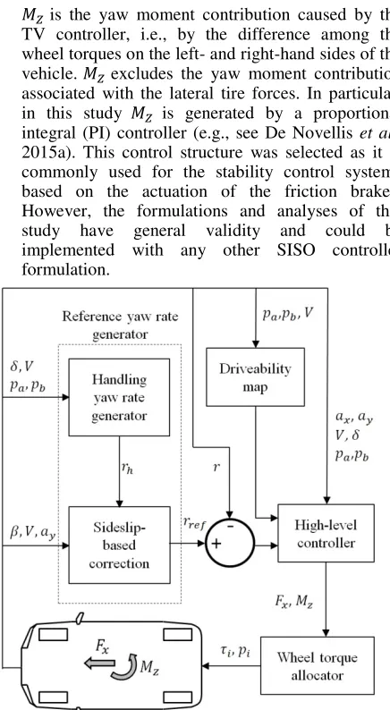
The simplified schematic of the vehicle control system is reported in Figure 1. The control structure consists of: i) A reference yaw rate generator. It defines the

so-called handling yaw rate, , aimed at enhancing the cornering response in steady-state conditions. Moreover, the reference yaw rate generator corrects

based on the actual sideslip angle, as detailed in Section 2.2.

is the yaw moment contribution caused by the TV controller, i.e., by the difference among the wheel torques on the left- and right-hand sides of the vehicle. excludes the yaw moment contribution associated with the lateral tire forces. In particular, in this study is generated by a proportional integral (PI) controller (e.g., see De Novellis et al., 2015a). This control structure was selected as it is commonly used for the stability control systems based on the actuation of the friction brakes. However, the formulations and analyses of this study have general validity and could be implemented with any other SISO controller formulation.

Figure 1. Simplified control structure schematic.

iii) A wheel torque control allocator, which outputs the reference torques, , and brake pressures, , for the individual wheels, corresponding to the values of and from the high-level controller. In the experimental tests of this study, the total drivetrain torques on the left- and right-hand sides of the vehicle, and , are calculated as:

= 0.5 −

= 0.5 +

(1)

where is the half-track width and is the wheel radius. Each wheel torque demand is then allocated to be 50% of the torque demand on the respective side. More advanced control allocation strategies could be adopted (Dizqah et al., 2016; Pennycott et al., 2014). However, a simple and predictable control allocation algorithm is ideal for the analysis

of this study, focused on the performance of the reference yaw rate generator and high-level controller.

2.2. Reference Yaw Rate Formulation

The key idea is to modify the reference yaw rate in critical conditions, i.e., when the sideslip angle is beyond predetermined thresholds. In this study is the output of a multi-dimensional look-up table (De Novellis et al., 2015a), based on: i) the driver inputs (i.e., steering wheel angle, ; accelerator and brake pedal positions, and ); ii) the measured or estimated vehicle states (e.g., vehicle speed, ; longitudinal acceleration, ). In particular, the design of modifies the cornering response of the vehicle: i) to reduce the understeer gradient with respect to the passive vehicle (i.e., the same vehicle plant without the TV controller); ii) to extend the region of linear cornering response; and iii) to extend the range of possible lateral accelerations for the available tire-road friction conditions. By means of a quasi-static model approach, the look-up table outputs different values of

depending on the driving mode selected by the driver, e.g., Normal Mode, Sport Mode, Enhanced Sport Mode, respectively characterized by increasing values of || for the same operating conditions (i.e., less understeering cornering behavior than the passive vehicle). In this study does not depend on the estimated tire-road friction coefficient, and is tuned for high tire-road friction conditions.

The steady-state value of the reference yaw rate,

!",$%, is given by:

!",$%= − &'− ($)

= '1 − &)+ &($ (2)

$ is the stability yaw rate, i.e., a yaw rate value that is

compatible with the current cornering conditions of the vehicle, corresponding to the measured lateral acceleration, ₊. The weighting factor, , is a linear function of the absolute value of the sideslip angle, ||, and is saturated between 0 and 1:

= ,

-._{|| −} 0 /0 || < 3%

3%

45− 3% /0 3% ≤ || ≤ 45

1 /0 || > 45

(3)

This means that for large values of || it is _!",$%=

'1 − &)+ &($, while for small values of || it is

!",$%= . 3% is the activation threshold, i.e., the

value of || below which no correction is applied to .

3% is set to 1 deg for all controller configurations discussed in Sections 4 and 5. ₄₅ is the limit threshold, i.e., the value of || above which _!",$%= '1 − &)+

respect to the one presented in (Lu et al., 2016a), which also takes into account the sideslip angle rate, 8. The parameters & and ( allow additional tuning freedom, however they are set to 1 in this study, i.e., _!",$%= _$ for high values of sideslip angle.

$ is calculated from its saturation value, _$%, which depends on ₊ , according to the steady-state relationship between yaw rate and lateral acceleration (Teng et al., 2015):

$%=+− 9/:;' +)<+ (4)

The parameter <₊ is used to provide some conservativeness on _$%, i.e., to ensure that the vehicle with a yaw rate equal to _$% is actually operating within its cornering limit. <₊ is set to 1 m/s2 in this study. In the practical tuning of the controller, <₊ can be defined as a function of =₊=.

$ is given by:

$= >_| /0 || < |$%|

$%|9/:;') /0 || ≥ |$%| (5)

Hence, _$ is the result of the saturation of according to the available friction conditions, defined by the measured lateral acceleration. The reference yaw rate,

!", which is input to the feedback yaw rate controller,

is calculated by filtering _!",$% , i.e., _!"'9) =

!",$%'9)/'1 + 9), where is the time constant of the first order filter and 9 is the Laplace operator.

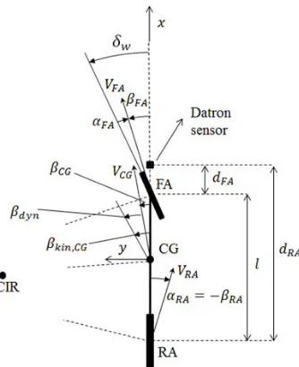
The value of in Equation (3) can be evaluated for any point along the A-axis of the vehicle reference system (see Figure 2, with the schematic of the vehicle cornering about its center of instantaneous rotation, CIR). The location at which is evaluated affects the performance of the TV controller because of the different kind of information contained in the sideslip value, as discussed later in this section.

Three cases are considered for : i) the front axle (FA), with the corresponding angle = _BC; ii) the center of gravity (CG), with the corresponding angle

= . This is the case normally discussed in the literature (for example, in (Teng et al., 2015)); and iii) the rear axle (RA), with the corresponding angle

= C. Note that the relationship between the sideslip angles calculated for two different points, D_E and D_F, located along the A-axis of the vehicle reference system, is given by:

GH = GI+

GIGH

GIcos GI

(6)

where _GIGH is the distance between D_E and D_F (positive if D_F is in front of D_E according to the conventions of this study), and _GI is the velocity of D_E.

The sideslip angle at a generic point D along the A

-axis, _G, can be split into two contributions, i.e., a kinematic contribution, _MN,G , and a dynamic contribution related to lateral tire slip, _O+N,G:

O+N,G= −G+ MN,G (7)

Figure 2. Top view of a single-track vehicle model with indication of the main parameters and variables.

During a cornering maneuver with zero tire slip angles on both axles (kinematic steering), e.g., in conditions of low speed maneuvering during parking, _O+N,G would be zero, and the vehicle would experience a sideslip angle equal to _MN,G. For example, if D ≡ Q&, _MN, in kinematic steering conditions can be calculated from the steering angle of the wheel, , i.e., through _MN,

≈

F/

≈

the trajectory radius at the centre of gravity (Genta, 1997).

This study adopts a different approach. In fact,

MN, is calculated starting from the measured yaw rate, :

MN, ≈ _≈F F (8)

In Equation (8) _MN, represents the sideslip angle that the vehicle would experience in kinematic steering conditions while cornering with its actual yaw rate, . As the actual steering response of a real vehicle is different from that of a neutral vehicle, the resulting value of _MN, differs from the one that can be calculated from the actual value of .

by imposing D_E≡ Q& and D_F≡ T in Equation (6), it results that _C= _O+N, therefore _C coincides with the dynamic vehicle sideslip angle, _O+N, computed through Equations (7) and (8).

The idea of considering _O+N= _C as control variable permits to constrain the net level of sideslip induced by the lateral slip of the rear tires, experiencing an average slip angle U_C= −_C. The rear axle is responsible for vehicle stability in cornering, i.e., the rear axle generates the stabilizing yaw moment that counteracts the destabilizing yaw moment caused by the steering action of the front tires. A large value of |_C| implies a rear axle that is operating at its limit, i.e., in critical conditions, potentially compromising the stability of the overall vehicle. As a consequence, a controller based on _O+N= _C intervenes when actually required in emergency conditions, and can be based on fixed thresholds, as significant values of _O+N represent a stability issue at any lateral acceleration, vehicle speed or tire-road friction condition. On the other hand, a controller based on would require variable thresholds, to prevent undesired interventions, e.g., caused by the significant values of _MN, during parking maneuvers with high values of , and hence low values of .

3. CONTROL SYSTEM DESIGN

Starting from the formulation of the single-track vehicle model (Genta, 1997; Milliken and Milliken, 1995) under the hypotheses of small steering angles, linear tire response and constant vehicle speed, the actual yaw rate, , can be expressed in the Laplace domain as:

'9) = & VW'9) '9) + & XY'9)'9) (9)

with:

& VW'9) =

Z VW'9)

['9) (10)

= \9 − ]^

_`\9F− a_`]^+ Z\b9 − Z^] + Z^\ + Z ]^

& XY=

Z XY'9)

['9)

(11)

= ZXY\9 + Z^]XY− ZXY]^

_`\9F− a_`]^+ Z\b9 − Z^] + Z^\ + Z ]^

where the stability derivatives are:

]^= QE+ QF, ] =Ic_d H, ]XY= −QE (12)

Z^= QE− eQF, Z = H_IfH_H

d ,

ZXY= −QE

(13)

Similarly, '9) can be obtained in the frequency domain as:

'9) = &^VW'9) '9) + &^XY'9)'9) (14)

with:

&^VW=

Z^VW'9)

['9) =]['9)− \ &^XY=

Z^XY'9)

['9)

=ZXY] − Z]XY− \ZXY+ _`]XY9

['9)

(15)

The front and rear cornering stiffness values for control system design, Q_E and Q_F, respectively of 37180 N/rad and 82690 N/rad, are those obtained from the detailed analysis in (Lu et al., 2016b), referred to the same vehicle demonstrator. They correspond to the vehicle operating at ₊= 8.3 m/s2 in high friction conditions.

The TV yaw moment is formulated as the output of a PI controller on the yaw rate error:

'g) = (hi !"'g) − 'g)j +

(k i !"'g) − 'g)j dg +

(k i`,$%'gc) − `'gc)j dg

(16)

(h, ( and ( are the proportional, integral and anti-windup gains. gc is the time value at the previous discretization step, and _`,$% is the saturated value of the reference yaw moment, set to 1600 Nm for all the experimental tests of the paper. Appropriate reset integrator conditions are included in the implemented controller formulation, see (De Novellis et al., 2015a; Lu et al., 2016b). In a first approximation, when neglecting the anti-windup, the control system design can be carried out by substituting the following transfer function into Equations (9) and (14):

'9) = QGm'9) i !"'9) − '9)j

= (h+(_{9 i} !"'9) − '9)j

(17)

Table 1. Control system parameters for (= 31623 Nm/rad.

A gain scheduling scheme is introduced for the proportional gain, (_h, with the aim of guaranteeing similar tracking bandwidth of the closed-loop system, regardless of vehicle speed. In this respect, for different speed values Table 1 shows: i) the natural frequency,

nN, and the damping ratio, o, of & VW'9) (note that

['9) can be expressed as ['9) = 9F+ 2 on_N9 + n_NF); Speed

(km/h)

(h

(Nms/rad) & V'9)

& VW'9)QGm'9)

Open-loop

& VW'9)QGm'9)

Closed-loop

nN

(HZ) o

&

(dB)

D

ii) the selected values of (_h; iii) the values of gain margin (&) and phase margin (D) of the open-loop transfer function, & _VW'9)Q_Gm'9); and iv) the tracking bandwidth (qr) of the closed-loop transfer function, i.e., & _VW'9)Q_Gm'9)/'1 + & _VW'9)Q_Gm'9)).

It is interesting to analyze the effects of the sideslip-based correction of the reference yaw rate, in particular when || > ₄₅and _!",$%= _$= ₊/ (<₊= 0 and

& = ( = 1 for simplicity). From the single-track model it is:

+= ' + 8) (18)

When substituting Equation (18) into Equation (16) (without considering the anti-windup term) and simplifying, 'g) becomes:

'g) = (h8'g) + ('g) (19)

which is the formulation of a proportional derivative (PD) regulator on 'g), i.e., Q_Gs'9), or, equivalently, a PI regulator on 8'g). This result is in agreement with the purpose of controlling 'g) . Moreover, by substituting Equation (19) into Equation (14) and re-arranging, '9) becomes:

'9) = &^XY,t'9)'9) =

Z^XY,t'9)

[t'9) '9) (20)

where:

Z^XY,t'9) = −_`]XY9 + Z]XY+ ZXY'\

− ]) (21)

[t'9) = −\_`9F+ 9a]^_`+ \Z − (hub

+ '−]^Z − aZ^+ (bu) (22)

The static gain of &_^XY,t is:

&^XY,t'9 = 0)

= Z]XY+ ZXY'\ − ])

'−]^Z − aZ^+ (b'\ − ]))

(23)

Consistently with Equation (19), &_^XY,t'9 = 0) does not depend on (_h, while it decreases with (, and tends to zero for (→ ∞. Similarly to Table 1, the stability of the response of the system in the sideslip tracking mode was verified through the analysis of the transfer function

&^VW'9)QGs'9).

4. EXPERIMENTAL SET-UP

4.1. The Vehicle Demonstrator

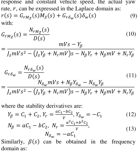
The experimental study was conducted on an electric Range Rover Evoque prototype (Figure 3), with four identical on-board drivetrains, each of them consisting of a switched reluctance electric motor (M1, M2, M3 and M4), a double-stage single-speed transmission system, constant velocity joints and a half-shaft. The vehicle prototype features a battery pack and a Vehicle Control Unit (VCU), which manages and coordinates all

the components, including the four inverters (I1, I2, I3 and I4). The pressure levels of the friction brakes are individually controlled by an electro-hydraulic braking system, set up during the European project E-VECTOORC (E-VECTOORC, 2016; Savitski et al., 2016). The TV controller detailed in Sections 2-3 was implemented on a dSPACE AutoBox system. The main vehicle parameters are reported in Table 2.

During the tests, the sideslip angle was measured through a Corrsys Datron S-350 sensor, installed on the front end of the car (see Figure 3). The values of sideslip angle for different points along the A-axis of the vehicle reference system were obtained through Equation (6), starting from the Datron measurement data, combined with the information from the 6-degree-of-freedom inertial measurement unit installed on the vehicle. Despite the availability of sideslip state estimators (e.g., see the one implemented in (De Novellis et al., 2015b)), the outputs from the Datron were used to calculate the sideslip control variable during the tests. This makes the controller comparison independent from the specificities of the sideslip angle estimation method, conferring reliability to this experimental proof of concept.

Figure 3. The vehicle demonstrator with the Corrsys Datron sideslip sensor installed on the front bumper (top); schematic of the electric drivetrain architecture (bottom).

Table 2. Main vehicle parameters.

Symbol Name and unit Value

\ Mass (kg) 2290

E Front semi-wheelbase (m) 1.399

S Wheelbase (m) 2.665

x Gearbox ratio (-) 10.56

Wheel radius (m) 0.364 2 Track width (m) 1.616

− No. of motors per axle (-) 2

O3 High-voltage dc bus level (V) 600 The following configurations of the vehicle demonstrator were considered during the tests:

M 1 M 2 I1

I2

δ

Battery Pack

Datron Sensor M 3

M 4

I3 VCU

• _{The baseline vehicle, PV, i.e., the passive vehicle}

with constant wheel torque distribution (25% of the total torque demand is assigned to each wheel).

• _{The TV-controlled vehicle without the}

sideslip-related variation of the reference yaw rate. This configuration is called AV, i.e., active vehicle, in Section 5.

• _{The TV-controlled vehicle with the sideslip-related}

variation of the reference yaw rate, based on _BC,

or _C, respectively corresponding to the test cases indicated as FA, CG and AVC-RA in the remainder. The values of ₄₅used for the AVC-FA, AVC-CG and AVC-RA are, respectively, 3 deg, 2 deg and 4 deg. They were selected through simulations and experiments in order to achieve good performance in the specific tests of this study. Interestingly, during the control system tuning, it was observed that an increase of

45 on the AVC-FA and AVC-CG cases brings vehicle stability issues in the two extreme maneuvers of this analysis.

• _{The controlled vehicle with constant electric}

drivetrain torque distribution (i.e., without TV control), but including direct yaw moment control through a stability control system based on the individual actuation of braking torques in emergency conditions. This is referred to as Electronic Stability Control (ESC) configuration in the remainder, and has similar functionality to that of conventional stability control systems of production passenger cars (van Zanten, 2000; Her et al., 2016). The emergency conditions are identified when = _!"− = > ∆_{% $}. _!" includes the sideslip-related variation, implemented as a function of _C. The value of the threshold, ∆_{% $}, is of ≈6 deg/s for the vehicle speed values of the relevant tests. The same PI controller gain design as for the TV-controlled cases is adopted for generating the reference yaw moment. The ESC yaw rate error for the PI controller is calculated by using a deadband of ±∆_{% $}, which is consistent with the activation condition of the stability control system. Moreover, the ESC mode reduces the traction torque demand – thus overruling the driver’s input – when this is considered necessary (i.e., based on = _!"− =) to improve the cornering safety by reducing vehicle speed.

4.2. Test Maneuvers

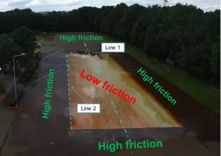
The proving ground located in Weert (Netherlands) was used for the experimental tests of this study. The test area consists of a surface that is 150 m long and 41 m

wide (Figure 4). The central part (50 m x 25 m) of such surface is characterized by a low friction area, made of epoxy and kept constantly wet by means of sprinklers. The remaining part of the proving ground is covered with common asphalt. The friction coefficient in the low friction area is ≈15% of the friction coefficient in the high friction area.

Two very demanding test maneuvers, called ‘Maneuver 1’ and ‘Maneuver 2’ in the remainder, were executed in the study. For both of them:

• _{The car is accelerated on a straight line until the}

reference speed value, ₅ (defined below), is steadily achieved.

• _{Once the vehicle is stabilized on 5, a constant}

wheel torque demand (100 Nm) is applied through the dSPACE system, thus bypassing driver’s input on the accelerator pedal.

• _{The vehicle executes a slalom maneuver with}

cones located at 20 m from each other on a straight line.

In particular:

• _{For Maneuver 1, the cones are located along line 1}

in Figure 4, i.e., the vehicle starts the test on the high friction area, then enters the low friction area, and, at the end of the maneuver, goes back into the high friction area.

• _{For Maneuver 2, the cones are located along line 2}

in Figure 4, i.e., on the border between the high friction surface and the low friction surface. As a consequence, the car experiences a continuous variation of tire-road friction conditions, which are different among the left and right tires of the vehicle during most of the test.

• _{5 is defined as the maximum initial speed at}

which the PV (i.e., the vehicle without TV controller) can complete the maneuver without hitting any cone. The value of ₅ is different for each test driver, and was determined through multiple tests.

Maneuver 1 and Maneuver 2 are particularly critical for stability control systems, because of the very swift variation of the tire-road friction coefficient, which requires prompt adaptation of the controller. Hence, these test conditions are even more demanding than those typically achievable in a uniformly low-friction proving ground, e.g., covered with snow/ice.

of the different TV controller set-ups. Each test was repeated several times with each driver. It was observed that the drivers generated quite variable steering wheel input profiles among each other for the same maneuver. However, no substantial variation of the vehicle performance trends was observed between the results associated to different drivers. In particular, the relative performance rating of the AV, AVC-FA, AVC-CG, AVC-RA and ESC cases did not change with the driver.

Figure 4. A drone view of the Weert proving ground, with indication of: i) the friction condition of the different surfaces; and ii) the two lines where cones were located for the execution of Maneuver 1 and Maneuver 2.

4.3. Performance Indicators

Six objective performance indicators are adopted for the assessment of each controller along the tests:

• _{The root mean square value of the yaw rate error,}

{u, which assesses the tracking performance of the feedback controller on yaw rate:

{u = |_g 1

"− gk ' !"'g) − 'g)) F_g %}

%~

(24)

where g and g_" represent the initial time and final time of the relevant part of the test, respectively.

g"− g is 10 s for Maneuver 1, and 5.5 s for Maneuver 2.

• _{The root mean square value of the difference}

between _!",$% and , i.e., {u_^, which assesses the significance of the intervention of the sideslip contribution of the controller, making _!",$% differ from :

{u^= |_g 1

"− gk ' !",$%'g) − 'g)) F_g %}

%~

(25)

• _{The maximum absolute value of sideslip angle at the}

rear axle, i.e., =_C,5= = =_O+N,5=.

• _{The normalized integral of the absolute value of the}

control action, €TQT, which evaluates the amount of direct yaw moment control effort:

€TQT =_g 1

"− g k |`'g)| %}

%~

g (26)

• ∆%_{, which provides the magnitude of the vehicle}

speed reduction during the test, expressed as a percentage of the initial speed, ₅:

∆% = 1005− ag "b

5 (27)

• _{The normalized integral of the absolute value of the}

steering wheel control action applied by the driver,

€T{QT. This indicator represents the steering wheel effort required for the successful completion of the test, i.e., for not hitting any cone:

€T{QT =_g 1

"− g k |'g)| %}

%~

g (28)

5. TEST RESULTS

This section presents a selection of the experimental test results on the Range Rover Evoque demonstrator along Maneuver 1 and Maneuver 2, including comparisons and analyses of the performance of the PV, the response of the same vehicle with the different TV controllers, and the behavior of the same vehicle with the ESC.

5.1. Maneuver 1

Figure 5 shows a visual comparison for the AV and AVC-FA cases along Maneuver 1, in the same spot of the low friction part of the test area. The frame was captured at a time g ≈ 7.5 s in the following Figures 6-10, reporting the time histories of the main variables. The oversteering problem of the AV, which requires the countersteering action of the driver, is evident in Figure 5. This is caused by the excessively high value of the reference yaw rate, designed for high friction conditions. The response of the AV is typical of a TV-controlled vehicle without a working friction estimator capable of modifying the reference value of yaw rate.

PV, while the AV spins. The instability of the AV is evident in Figures 6 and 7, where, after ≈8.5 s, the sideslip angle has opposite sign with respect to the yaw rate. Figures 9 and 10 report the average slip angles of the front and rear axles. In particular, the front slip angle, U_BC, is calculated from the front sideslip angle and average steering angle, i.e., U_BC= − _BC. From 0 s to 4 s, the slip angle at the front axle tends to be larger in magnitude than the slip angle at the rear axle for all cases, i.e., the vehicle tends to understeer. After 4 s, the PV and AV present a rear slip angle significantly larger (in magnitude) than the front slip angle, i.e., they show an oversteering behavior, differently from the AVC cases.

Based on this qualitative analysis, the first important conclusion is that in variable friction conditions it is much more important to have appropriate and swiftly adaptable generation of the reference yaw rate signal, rather than an advanced controller providing excellent tracking performance. Moreover, a TV-controlled vehicle that is not properly tuned for low or variable friction conditions is potentially more dangerous than a passive vehicle.

Figure 5. Visual comparison for Maneuver 1, when the vehicle is slaloming in the low friction surface: AV (left), AVC-FA (right) – frame captured at g ≈7.5 s in Figures 6-10.

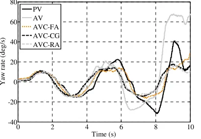
Figure 6. Maneuver 1, driver A: 'g) for different vehicle controller configurations.

Figure 7. Maneuver 1, driver A: _BC'g) for different vehicle controller configurations.

Figure 8. Maneuver 1, driver A: 'g) for different vehicle controller configurations.

More specifically, Figures 6-10, together with Table 3, allow objective comparisons of the performance of the different control system configurations. Among the AVCs, the AVC-RA case provides: i) smoother and slightly lower profile of |'g)| (Figure 6); ii) smaller values of || (see Figures 5, 7, 8 and 10), not only at the rear axle, but at the front axle and center of gravity as well, despite ₄₅ being smaller for the AVC-FA and AVC-CG cases; iii) the best yaw rate tracking performance, with a {u of 3.4 deg/s, against the 5.2 deg/s and 4.0 deg/s of the AVC-FA and AVC-CG (Table 3); iv) the lowest intervention of the sideslip-based correction, which is evident from a {u_^ of only 0.83 deg/s, against the 4.7 deg/s and 1.0 deg/s of the AVC-FA and AVC-CG cases. On the other hand, this is associated with a slightly increased control effort (see the €TQT values in Table 3); and v) the smallest vehicle speed reduction, ∆%, which is 5.2% for the AVC-RA, against the 6.5% of the other two AVC cases (Table 3).

As a consequence, for Maneuver 1 the AVC-RA appears to be the best AVC option, and these

0 2 4 6 8 10

-40 -20 0 20 40 60 80

Time (s)

Y

aw

r

at

e

(d

eg

/s

)

PV AV AVC-FA AVC-CG AVC-RA

0 2 4 6 8 10

-10 -5 0 5 10 15

Time (s)

S

id

es

li

p

a

n

g

le

(

d

eg

)

PV AV AVC-FA AVC-CG AVC-RA

0 2 4 6 8 10

-10 -5 0 5 10 15

Time (s)

S

id

es

li

p

a

n

g

le

(

d

eg

)

experiments validate the AVC-RA idea described in Section 2.2. In fact, the sideslip-based correction of the AVC-RA intervenes less, and only when it is really needed, i.e., when there is a significant dynamic sideslip angle. In the AVC-FA and AVC-CG the correction intervenes also when there is a large value of steering input from the driver and a large trajectory curvature (i.e., a significant kinematic sideslip angle), which does not necessarily result into safety-critical vehicle operation.

Figure 9. Maneuver 1, driver A: U_BC'g) for different vehicle controller configurations.

Figure 10. Maneuver 1, driver A: U_C'g) = −_C'g) for different vehicle controller configurations.

Table 3. Performance indicators for Maneuver 1, driver A, ₅= 37 km/h.

Case {u

(deg/s)

{u^

(deg/s)

=C,5=

(deg)

€TQT

(Nm) ∆V%

€T{QT

(deg) PV 17.9 NA 13.0 0 21.3 54.4 AV 47.1 NA 85.6 1224 56.1 87.8 AVC-FA 5.2 4.7 6.8 822 6.5 35.1 AVC-CG 4.0 1.0 4.7 953 6.5 28.1 AVC-RA 3.4 0.83 3.1 1013 5.2 29.0

5.2. Maneuver 2

Similar results to those discussed in detail for Maneuver 1 were obtained for Maneuver 2 (see Figures 11-15 and

Table 4), with the controller based on _C consistently outperforming the other options. Actually, the AVC-RA case is the only one capable of maintaining the rear axle sideslip angle (i.e., the dynamic sideslip angle) within limits that are typical of normal driving conditions. In fact, the AVC-RA case achieves a =_C,5= value of 3.3 deg (Table 4), while the other AVC cases are characterized by =_C,5= >10 deg.

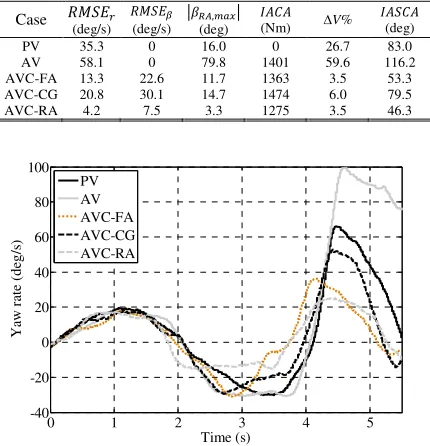
Table 4. Performance indicators for Maneuver 2, driver B, ₅= 43 km/h.

Case {u

(deg/s)

{u^

(deg/s)

=C,5=

(deg)

€TQT

(Nm) ∆V%

€T{QT

(deg) PV 35.3 0 16.0 0 26.7 83.0 AV 58.1 0 79.8 1401 59.6 116.2 AVC-FA 13.3 22.6 11.7 1363 3.5 53.3 AVC-CG 20.8 30.1 14.7 1474 6.0 79.5 AVC-RA 4.2 7.5 3.3 1275 3.5 46.3

Figure 11. Maneuver 2, driver B: 'g) for different vehicle controller configurations.

Figure 12. Maneuver 2, driver B: U_C= −_C'g) for different vehicle controller configurations.

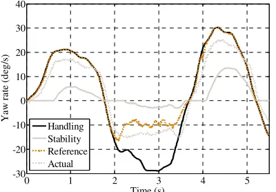
In order to analyze the effect of the sideslip-based correction in detail, Figures 14 and 15 show the four relevant yaw rates, i.e., 'g), _$'g), _!"'g) and 'g), and the corresponding yaw moment, for the AVC-RA case. At the beginning of the maneuver (between 0 and

0 2 4 6 8 10

-8 -6 -4 -2 0 2 4 6 8 Time (s) S li p a n g le a t fr o n t a x le ( d e g ) PV AV AVC-FA AVC-CG AVC-RA

0 2 4 6 8 10

-20 0 20 40 60 80 Time (s) S li p a n g le a t re ar a x le ( d eg ) PV AV AVC-FA AVC-CG

AVC-RA -400 1 2 3 4 5

-20 0 20 40 60 80 100 Time (s) Y aw r at e (d eg /s ) PV AV AVC-FA AVC-CG AVC-RA

0 1 2 3 4 5

≈ 1.8 s), when the outer wheels are on the high friction area, |_C| is small and _!" is greater than the actual yaw rate, resulting in a positive (destabilizing) yaw moment. Just before entering the low friction area (between ≈1.8 s and ≈2 s), the reference yaw rate becomes lower than the actual one, resulting in a negative yaw moment, which is firstly stabilizing (when the vehicle is still turning left) and then destabilizing (when vehicle starts turning right). Immediately after entering the low friction area with the outer wheels (at

≈ 2 s), |_C| increases significantly and the sideslip-based correction intervenes, i.e., the reference yaw rate gets closer to the stability yaw rate, thus becoming greater (i.e., less negative) than the actual yaw rate, implying a positive (stabilizing) yaw moment. After 3.5 s the cornering action is carried out with the outer wheels operating in high friction conditions. As discussed for the initial part of the maneuver (before 2 s), this is associated with small values of |_C|, and therefore no correction of the handling yaw rate is needed.

Figure 13. Maneuver 2, driver B: 'g) for different vehicle controller configurations.

Figure 14. Maneuver 2, driver B: overlap of the different yaw rates (handling, stability, reference and actual) for the AVC-RA case.

Figure 15. Maneuver 2, driver B: yaw moment for the AVC-RA case.

5.3. Comparison of AVC-RA and ESC

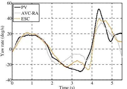
This section compares the PV, AVC-RA and ESC configurations along Maneuver 1 and Maneuver 2. The objective is to assess the vehicle safety benefit that is achievable through continuously active TV control, with respect to an ESC system operating only in emergency conditions.

Figures 16 and 17 report the time histories of vehicle yaw rate and sideslip angle along Maneuver 2. Tables 5 and 6 include the performance indicators for Maneuver 1 and Maneuver 2, with the vehicle operated respectively by driver C and driver D. In Table 5 the

€T{QT values are larger than in Table 3, since driver C managed to execute the test at larger values of initial vehicle speed than driver A. On the other hand, in Table 6 the €T{QT values are larger than in Table 4, despite

5 is the same, because of the lack of specific training of driver D, who executed the tests in Table 6. In both cases the ESC provides a performance level that is intermediate between that of the PV and AVC-RA cases. The continuous operation of the TV controller of the AVC-RA allows prompt limitation of the peaks and overshoots of vehicle yaw rate and rear slip angle, which follow each steering wheel input. The specific ESC tuning struggles recovering the vehicle yaw dynamics, as it intervenes when the vehicle is already quite far from its reference cornering behavior.

Future analyses will include sensitivity studies on the ESC gains and yaw moment saturation value. In any case, given the very low friction value of the section of the proving ground covered with Epoxy, it is not recommended to significantly increase the ESC control gains or the yaw moment saturation level, as these modifications could trigger wheel slip control issues and aggressive interventions of the anti-lock braking system.

0 1 2 3 4 5

-400 -300 -200 -100 0 100 200 300 400

Time (s)

δ (

d

eg

)

PV AV AVC-FA AVC-CG AVC-RA

0 1 2 3 4 5

-30 -20 -10 0 10 20 30 40

Time (s)

Y

a

w

r

a

te

(

d

eg

/s

)

Handling Stability Reference Actual

Y

aw

m

o

m

en

t

(N

m

Figure 16. Maneuver 2, driver D: 'g) for different vehicle controller configurations.

Figure 17. Maneuver 2, driver D: _C'g) for different vehicle controller configurations.

Table 5. Performance indicators for Maneuver 1, driver C, ₅= 42 km/h.

Case {u

(deg/s)

{u^

(deg/s)

=C,5=

(deg)

€TQT

(Nm) ∆V%

€T{QT

(deg) PV 13.4 0 9.1 0 26.5 52.2 AVC-RA 4.6 4.5 3.5 1081 6.0 41.1 AVC-ESC 11.0 6.8 8.3 583 26.2 51.8 Table 6. Performance indicators for Maneuver 2, driver D, ₅= 43 km/h.

Case {u_(deg/s) {u_(deg/s) ^ =C,5_(deg) = €TQT_(Nm) ∆V% €T{QT

(deg) PV 29.3 0 14.2 0 16.7 82.1 AVC-RA 5.3 12.7 4.6 1337 3.5 63.3 AVC-ESC 11.5 15.1 8.0 623 13.3 69.8

6. CONCLUSIONS

The analysis presented in this paper leads to the following conclusions:

• _{In specific maneuvers tested at the Weert proving}

ground, continuously active torque-vectoring control based on yaw rate feedback, without proper adaptability to swiftly variable tire-road friction

conditions, can bring more safety-critical vehicle response than that of a passive vehicle without any form of direct yaw moment control.

• _{Effective continuous control of yaw rate with}

sideslip angle limitation is achievable with a single input single output yaw-rate-based control structure, where the reference yaw rate is modified according to the measured (or estimated) sideslip angle.

• _{The proposed controller formulation works as a PI}

yaw rate controller when the reference yaw rate coincides with the handling yaw rate, and as a PD controller on sideslip angle when the reference yaw rate coincides with the saturation value of the stability yaw rate.

• _{The sideslip-based weighting function between the}

handling yaw rate and the stability yaw rate allows controller adaptability to very quick and non-uniform variations of the tire-road friction coefficient on the individual tires. Its tuning is essential to define vehicle response on variable friction surfaces.

• _{Based on the experimental results it is recommended}

to control the dynamic sideslip angle, which (in absolute value) is coincident with the sideslip angle at the rear axle, i.e., the average slip angle of the rear tires. In fact, the control system performance based on sideslip angle limitation at the front axle or at the vehicle center of gravity (which is the common option in the literature) is shown to be significantly weaker in the specific tests, and can also lead to undesired control system interventions if it is not carefully tuned for large steering angle values.

• _{The continuous actuation of direct yaw moment}

control through torque-vectoring brings significant benefits in limiting yaw rate overshoots in very low or quickly variable friction conditions, thus providing safer performance than that of the case study stability control system based on braking torque actuation only in emergency conditions.

ACKNOWLEDGEMENT −−−− The research leading to these results has received funding from the European Union Seventh Framework Programme FP7/2007-2013 under Grant Agreement No. 608897 (iCOMPOSE project).

REFERENCES

Abe M., Kano Y., Suzuki K., Shibahata Y., Furukawa Y. (2001). Side-slip control to stabilize vehicle lateral motion by direct yaw moment, JSAE review, Vol. 22(4), pp. 413-419.

Baffet G., Charara A., Stephant J. (2006). Sideslip angle, lateral tire force and road friction estimation in

0 1 2 3 4 5

-40 -20 0 20 40 60

Time (s)

Y

aw

r

at

e

(d

eg

/s

)

PV AVC-RA ESC

0 1 2 3 4 5

-5 0 5 10 15

Time (s)

S

id

es

li

p

a

n

g

le

a

t

re

ar

a

x

le

(

d

eg

) PV_AVC-RA

simulations and experiments, IEEE International Conference on Control Applications.

De Novellis L., Sorniotti A., Gruber P. (2015a). Driving modes for designing the cornering response of fully electric vehicles with multiple motors, Mechanical Systems and Signal Processing, Vol. 64-65, pp. 1-15.

De Novellis L., Sorniotti A., Gruber P., Orus J., Fortun J.M.R., Theunissen J., De Smet J. (2015b). Direct yaw moment control actuated through electric drivetrains and friction brakes: theoretical design and experimental assessment, Mechatronics, Vol. 26, pp. 1-15.

De Novellis L., Sorniotti A., Gruber P. (2014a). Wheel torque distribution criteria for electric vehicles with torque-vectoring differentials, IEEE Transactions on Vehicular Technology, Vol. 63(4), pp. 1593-1602.

De Novellis L., Sorniotti A., Gruber P., Pennycott A. (2014b). Comparison of feedback control techniques for torque-vectoring control of fully electric vehicles, IEEE Transactions on Vehicular Technology, Vol. 63(8), pp. 3612-3623.

Di Cairano S., Tseng, D. Bernardini H.E., Bemporad A. (2013). Vehicle yaw stability control by coordinated active front steering and differential braking in the tire sideslip angles domain, IEEE Transactions on Control Systems Technology, Vol. 21(4), pp. 1236-1248.

Dizqah A.M., Lenzo B., Sorniotti A., Gruber P., Fallah S., De Smet J. (2016). A fast and parametric torque distribution strategy for four-wheel-drive energy-efficient electric vehicles, IEEE Transactions on Industrial Electronics, Vol. 63(7), pp. 4367-4376.

Esmailzadeh E., Goodarzi A., Vossoughi G.R. (2003). Optimal yaw moment control law for improved vehicle handling, Mechatronics, Vol. 13(7), pp. 659–675.

E-VECTOORC, www.e-vectoorc.eu, last accessed on 19th August 2016.

Geng C., Mostefai L., Denaï M., Hori Y. (2009). Direct yaw-moment control of an in-wheel-motored electric vehicle based on body slip angle fuzzy observer, IEEE Transactions on Industrial Electronics, Vol. 56(5), pp. 1411-1419.

Genta G. (1997). Motor vehicle dynamics: modeling and simulation, World Scientific, Vol. 43.

Graber J. (1997). Driving stability controller with coefficient of friction dependent limitation of the reference yaw rate, U.S. Patent No. 5,671,143.

Hahn J.O., Rajamani R., Alexander L. (2002). GPS-based real-time identification of tire-road friction coefficient, IEEE Transactions on Control System Technology, Vol. 18(3), pp. 331-343.

Her H., Koh Y., Joa E., Yi K., Kim K.. (2016). An integrated control of differential braking, front/rear traction, and active roll moment for limit handling performance, IEEE Transactions on Vehicular Technology, Vol. 65(6), pp. 4288-4300.

Hsu Y.J., Laws S.M., Gerdes J.C. (2010). Estimation of tire slip angle and friction limits using steering torque, IEEE Transactions on Control System Technology, Vol. 18(4), pp. 896-907.

Kaiser G. (2014). Torque Vectoring - Linear Parameter-Varying Control for an Electric Vehicle, Hamburg-Harburg Technical University, PhD thesis.

Kim C.S., Hahn J.O., Hong K.S, Yoo W.S. (2015). Estimation of Tire–Road Friction Based on Onboard 6-DoF Acceleration Measurement, IEEE Transactions on Vehicular Technology, Vol. 64(8), pp. 3368-3377.

Liu C.S., Peng H. (1996). Road friction coefficient estimation for vehicle path prediction, Vehicle system dynamics, Vol. 25(S1), pp. 413-425.

Lu Q., Gentile P., Tota A., Sorniotti A., Gruber P., Costamagna F., De Smet J. (2016a). Enhancing vehicle cornering limit through sideslip and yaw rate control, Mechanical Systems and Signal Processing, Vol. 75, pp. 455-472.

Lu Q., Sorniotti A., Gruber P., Theunissen J., De Smet J. (2016b). H∞ loop shaping for the

torque-vectoring control of electric vehicles: theoretical design and experimental assessment, Mechatronics, Vol. 35, pp. 32-43.

Manning W.J., Crolla D.A. (2007). A review of yaw rate and sideslip controllers for passenger vehicles, Transactions of the Institute of Measurement and Control, Vol. 29(2), pp. 117-135.

Milliken W.F., Milliken D.L. (1995). Race Car Vehicle Dynamics, SAE International.

Pennycott A., De Novellis L., Sabbatini A., Gruber P., Sorniotti A. (2014). Reducing the motor power losses of a four-wheel-drive, fully electric vehicle via wheel torque allocation, Proceedings of the Institution of Mechanical Engineers, Part D: Journal of Automobile Engineering, Vol. 228(7), pp. 830-839.

Ray L.R. (1997). Nonlinear tire force estimation and road friction identification: simulation and experiments, Automatica, Vol. 33(10), pp. 1819-1833.

Savitski D., Ivanov V., Shyrokau B., Puetz T., De Smet J. (2016). Experimental investigations on continuous regenerative anti-lock braking system of full electric vehicle, International Journal of Automotive Technology, Vol. 17(2), pp. 327-338.

Skogestad S., Postlethwaite I. (2005). Multivariable feedback control, Wiley.

Tchamna R., Youn I. (2013). Yaw rate and side-slip control considering vehicle longitudinal dynamics, International Journal of Automotive Technology, Vol. 14(1), pp.53-60.

Teng G.W., Xiong L., Leng B., Hu S.L. (2015). A novel reference model for vehicle dynamics control, 24th International Symposium on Dynamics of Vehicles on Roads and Tracks (IAVSD).

Integrated optimal dynamics control of 4WD4WS electric ground vehicle with tire-road frictional coefficient estimation, Mechanical Systems and Signal Processing, Vol. 60, pp.727-741.