DCT and DST based Image Compression for 3D Reconstruction

DCT and DST based Image Compression for 3D

Reconstruction

SIDDEQ, Mohammed and RODRIGUES, Marcos

<http://orcid.org/0000-0002-6083-1303>

Available from Sheffield Hallam University Research Archive (SHURA) at:

http://shura.shu.ac.uk/15146/

This document is the author deposited version. You are advised to consult the

publisher's version if you wish to cite from it.

Published version

SIDDEQ, Mohammed and RODRIGUES, Marcos (2017). DCT and DST based

Image Compression for 3D Reconstruction. 3D Research, 8 (5), 1-19.

Copyright and re-use policy

See

http://shura.shu.ac.uk/information.html

1

DCT and DST based Image Compression for 3D Reconstruction

Mohammed M. Siddeq and Marcos A. Rodrigues GMPR-Geometric Modelling and Pattern Recognition Research Group,

Sheffield Hallam University, Sheffield, UK [email protected], [email protected]

Abstract

This paper introduces a new method for 2D image compression whose quality is demonstrated through accurate 3D reconstruction using structured light techniques and 3D reconstruction from multiple viewpoints. The method is based on two discrete transforms: 1) A one-dimensional Discrete Cosine Transform (DCT) is applied to each row of the image. 2) The output from the previous step is transformed again by a one-dimensional Discrete Sine Transform (DST), which is applied to each column of data generating new sets of high-frequency components followed by quantization of the higher frequencies. The output is then divided into two parts where the low-frequency components are compressed by arithmetic coding and the high frequency ones by an efficient minimization encoding algorithm. At decompression stage, a binary search algorithm is used to recover the original high frequency components. The technique is demonstrated by compressing 2D images up to 99% compression ratio. The decompressed images, which include images with structured light patterns for 3D reconstruction and from multiple viewpoints, are of high perceptual quality yielding accurate 3D reconstruction. Perceptual assessment and objective quality of compression are compared with JPEG and JPEG2000 through 2D and 3D RMSE. Results show that the proposed compression method is superior to both JPEG and JPEG2000 concerning 3D reconstruction, and with equivalent perceptual quality to JPEG2000.

Keywords: DCT, DST, High Frequency Minimization, Binary Search Algorithm

1.

Introduction

Transform coding is at the heart of the majority 2D image/video coding systems and standards. Spatial image data (image samples or motion-compensated residual samples) are transformed into a different representation, the transform domain. There are good reasons for transforming image data in this way. Spatial image data is inherently ‘difficult’ to compress; neighbouring samples are highly correlated and the energy tends to be evenly distributed across an image, making it difficult to discard data or reduce the precision of data without adversely affecting image quality [1,2].With a suitable choice of transform, the data becomes ‘easier’ to compress in the transform domain. There are several desirable properties of a transform for compression. It should compact the energy in the image, i.e., concentrate the energy into a small number of significant values; it should de-correlate the data so that discarding ‘insignificant’ data – normally high frequency data – has a minimal effect on image quality; and it should be suitable for practical implementation in software and hardware [3,4].

The two most widely used image compression transforms are the discrete cosine transform (DCT) and the discrete wavelet transform (DWT) [3,4,5]. The DCT is usually applied to small, regular blocks of image samples (e.g. 8x8 squares) and the DWT is usually applied to larger image sections or to complete images. Many alternatives have been proposed, for example 3D transforms (dealing with spatial and temporal correlation), variable block size transforms, fractal transforms, and Gabor analysis. The DCT has proved particularly useful and it is at the core of most current generation of image and video coding standards, including JPEG, H.261, H.263, H.263+, MPEG-l, MPEG-2 and MPEG-4 [6,7].

2

and connectivity of a 3D mesh can be tackled by several techniques such as high degree polynomial interpolation [13] or partial differential equations [19,20], the issue of efficient compression of 2D images both for 3D reconstruction and texture mapping has not yet been addressed in a satisfactory manner. Moreover, in most applications that share common data, it is necessary to transmit 3D models over the Internet. For example, to share CAD/CAM assets, e-commerce applications, update content for entertainment applications, or to support collaborative design, analysis, display of engineering, medical and scientific datasets. Bandwidth imposes hard limits on the amount of data transmission and, together with storage costs calls for more efficient 3D data compression for exchange over the Internet and other networked environments. Using structured light techniques for 3D reconstruction, surface patches can be compressed as a 2D image together with 3D calibration parameters, transmitted over a network and remotely reconstructed (geometry, connectivity and texture map) at the receiving end with the same resolution as the original data [15, 21].

Related to the techniques proposed in this paper, our previous work on data compression is summarized as follows:1) Focused on compressing structured light images for 3D reconstruction, Siddeq and Rodrigues [15]proposed a method in 2014 where a single level DWT is followed by a DCT on the LL sub-band yielding the DC component and the AC-matrix. A second DWT is applied to the DC components whose second level LL2 sub-band is transformed again by DCT. A matrix minimization algorithm was applied to the AC-matrix and other sub-bands. Compression ratios of up to 98% were achieved. 2) Siddeq and Rodrigues in same year [16], proposed technique where a DWT was applied to variant arrangements of data blocks followed by arithmetic coding. The novel aspect of that paper is at decompression stage, where a Parallel Sequential Search Algorithm was proposed and demonstrated. Compression ratios of up to 98.8% were achieved. 3) In Siddeq and Rodrigues[18] a two-level DWT was applied followed by a DCT to generate a DC-component array and an MA-Matrix (Multi-Array Matrix). The MA-Matrix was then partitioned into blocks and a minimization algorithm coded each block followed by the removal of zero valued coefficients and arithmetic coding. At decompression stage, a new algorithm called Fast-Match-Search decompression was used to reconstruct the high-frequency matrices by computing data probabilities through a binary search algorithm in association with a look up table. A comparative analysis of various combinations of DWT and DCT block sizes was performed, with compression ratios up to 99.5%.

3

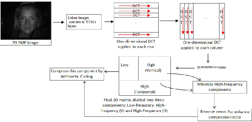
In this paper, we introduce a new method based on DCT and DST for compressing 2D images with structured light patterns for 3D surface reconstruction (i.e., the 2D images have embedded stripe patterns, and the detection and processing of such patterns are used to generate a 3D surface). Additionally, the method is applied to a series of 2D images (with no structured light patterns) and used to convert from multiple 2D images to a 3D surface [26]. Following the discrete transformations, a high-frequency minimization method is used to convert each three adjacent coefficients to a single integer, reducing the data size to a third of its original size. The final step is to apply arithmetic coding to the reduced data. The main steps in the compression algorithm are depicted in Figure 1.

2. Using One-Dimensional Discrete Cosine Transform (DCT)

The one-dimensional DCT is used to transform each row from an image (spatial domain) to obtain transform image called "Tdct", a shown in the following [3,4,5]:

Tdct(i) =



 











2

)

1

2

(

cos

)

(

)

(

2

n

i

t

t

I

i

C

n



I(t) =













 

n

j

t

j

T

j

C

n

2

)

1

2

(

cos

)

(

)

(

2



where\ C(i)

        0 , 1 0 , 2 1/2

i if

i if

Where i=0, 1, 2, 3, …, n-1 represents images row size from “I”, and the output is a set of DCT coefficients "Tdct". The first coefficient is called DC coefficient, and the rest are referred to as the AC coefficients. Notice that the coefficients are real numbers, and they are rounded off to integers. The important feature of the DCT is that it is useful in image compression [14]. It takes correlated input data and concentrates its energy in just the first few transform coefficients. If the input data consists of correlated quantities, then most of the "n" transform coefficients produced by the DCT are zeros or small numbers [8], and only a few are large (normally the first data). The early coefficients contain the most important (low-frequency) image information and the later coefficients contain the less-important (high-frequency) image information [6,17]. This feature allows good compression performance as a proportion of the less important coefficient scan be discarded without much degradation of image quality. Figure 2 shows the DCT applied to each row of a small image size 8x8 without using scalar quantization.

Original data ( image data) Tdct : DCT applied to each row

4

Figure 2. (Left) Original block of data, (right) Tdct produced by DCT.

3. One Dimensional Discrete Sine Transform (DST)

Our research has indicated that a one dimensional DCT works together with a one-dimensional DST yielding large amounts of high-frequency components. These high frequency components are useful to obtain high compression ratios comparable to the JPEG technique. In this research, we will apply one dimensional DST to each column of the transformed matrix "Tdct" from previous section. The DST

definition is represented as follows [8,9]:



(



k=1,2,…N



(



Equation (3) is used to transform "n" values of "Tdct" matrix into "n" coefficients. These are the low and high frequency coefficients containing important and less important image information. The one-dimensional DST is applied to each column of "Tdct" to produce a new transformed matrix "Tdst". The DST is equivalent to the imaginary part of the Discrete Fourier Transformation (DFT) and the results of the DST are real numbers [10,11]. The main advantage of using the DST for image compression in this context is that the DST preservers the image quality encoded by the low frequency components of "Tdct" and increases the number of zeros, which can be discarded without loss of quality.

After the DST, we apply a quantization of the high frequency components of the transformed matrix "Tdst". In this way, the quantization means losing only insignificant information from the matrix. Each coefficient in the matrix is divided by the corresponding number from a “Quantization table” and the result is rounded off to the nearest integer. The following equation is proposed as a quantization table.

Q(i,j)=(i+j) * F (5)

Where: F>0 and i,j=1,2,3,...,n x m (image dimensions)

5

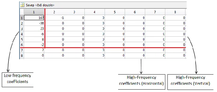
Figure 3. DST applied to each Column of Tdct followed by quantization with F=2 (See Equation (5))

In the above example, low and high frequency components are determined by the user. The low-frequency ones are not compressed any further, we just represent them in fewer bytes by arithmetic coding. Meanwhile, the high-frequency components either horizontal or vertical are compressed by the High-Frequency Minimization algorithm described in the next section.

4. High Frequency Minimization Algorithm

In this section, we describe an algorithm to convert the high-frequency coefficients (i.e. from previous section results passed to Minimization algorithm) into a compressed array called Minimized-Array through a matrix minimization method involving eliminating zeros and triplet encoding whose output is then subjected to arithmetic coding. Normally, the high frequency components contain large numbers of zeroes with a few nonzero data. The technique eliminates zeroes and enhances compression ratio [14, 15, 16, 17, 18].

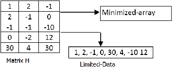
The high-frequency minimization algorithm is applied further reducing the size of high-frequency sub-matrix by 2/3.This process hinges on defining three key values and multiplying these by three adjacent entries in H (the matrix of high frequency coefficients) which are then summed over producing single integer values as shown in Figure 4 [16, 18].

Figure 4: High-Frequency Minimization Algorithm used to compress coefficients (D1, D2…, Dnm) from matrix H

6

Thus, each set of the three entries from H are converted into a single value which are then stored into a new coded array (Minimized-Array). Assuming that 𝑁 is the length of H, 𝑖 = 1,2, … , 𝑁 − 3, and 𝑗 is the index of new coded array, the following transformations define the high frequency encoding[15-18]:

𝑴𝒊𝒏𝒊𝒎𝒊𝒛𝒆𝒅_𝑨𝒓𝒓𝒂𝒚𝒋= 𝐾1𝑯𝑖+ 𝐾2𝑯(𝑖+1)+ 𝐾3𝑯(𝑖+2) (4)

The key values 𝐾1, 𝐾2, 𝐾3are generated by a key generator algorithm as in [17,18] described through Equations 5, 6, 7 and 8 below. Because the keys are data-dependent of max(H), each matrix will have their unique set of keys if their max(H) are distinct. 𝑀 = 1.5 max(𝑯) (5)

𝐾1= 1 (6)

𝐾2= 𝐾1+ 𝑀 + 𝐹𝑎𝑐𝑡𝑜𝑟 (7)

𝐾3= 𝐹𝑎𝑐𝑡𝑜𝑟 ∗ 𝑀(𝐾1+ 𝐾2) (8)

Where 𝐹𝑎𝑐𝑡𝑜𝑟 ≥ 1 and K1≥ 1are integer values. The quantity Factor is a scaling factor to enlarge the

degree of separation between the 3 generated keys. The keys themselves are the weights of each triplet summation in the minimized-array. The original values of each triplet can later be recovered by estimating the H values (See Section 5) for that Minimized-Array. Following the models above, the Minimized-Array for the example in Figure 3 can be illustrated in the following Table 1.

Table 1: From the example of Figure 3: each high-frequency sub-matrix is compressed independently

Assume M=2 (Maximum value in high-frequency sub-matrix: Horizontal) , the Keys values will be: K1=1, K2=5, K3=18 for both high-frequencies components: Horizontal and Vertical

High-Frequency Sub-matrix Compressed Size Comments

Minimized-Array(Vertical)={-1,0,0, 0, ... 0} compressed size 16 48(original size)/3 =16 data

Minimized-Array(Horizontal)={2,0,0, 0,0,0} compressed size 6 16(original size)/3 = 5.3 (last zero is alone)

Our compression method creates a new array of header data H, which is used later by the decompression algorithm to estimate the original data values. This information is kept in the header of the compressed file as a string. Figure 5 below illustrates the concept through a numerical example.

Figure 5: Limited-Data appearing in 𝑯 are kept in the header file for recovery.

7

The encoded triplets in the Minimized-Array may contain large number of zeros which can be further encoded through a process proposed by [18]. For example, assume the following encoded Minimized-Array={125, 0, 0,0,73, 0, 0,0,0,0, -17}.The zero array will be {0,3,0,5,0} where the zeros in red refer to nonzero data existing at these positions and the numbers in black refer to the number of zeros between two consecutive non-zero data. To increase the compression ratio, the number 5 can be broken up into 3 and 2 to increase data redundancy. Thus, the equivalent zero array would be {0,3, 0, 3, 2, 0} and the nonzero array would be {125,73,-17}. According to this method, the Minimized-Array both Horizontal and Vertical can be illustrated in Table 2.

Table 2: Each Minimized-Array is coded to zero-array and nonzero-array

High-Frequency Sub-matrix Zero-Array Nonzero-Array

Minimized-Array(Vertical)={-1,0,0, 0 ... 0} Zero(Vertical)={0,5, 5, 5} Nonzero-Array(Vertical)={-1}

Minimized-Array(Horizontal)={2,0,0, 0,0, 0} Zero(Horizontal)={0, 5} Nonzero-Array(Horizontal)={2}

Note: the "0" refers to the nonzero data in Nonzero-Arrays

The final step of compression is arithmetic coding which computes the probability of all data and assigns a range to each data (low and high) to generate streams of compressed bits [5].The arithmetic coding applied here takes a stream of data and converts into a single floating point value. The output is in the range between zero and one that, when decoded, returns the exact original stream of data.

5. The Fast-Matching Search Decompression Algorithm

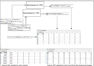
The decompression algorithm is the inverse of compression. First, decode the Minimized-Array for both horizontal and vertical components by combining the zero-array with the non-zero-array. Second, decode high-frequencies from the Minimized-Array using the fast matching search (FMS) algorithm [18]. Third, inverse the DST and DCT to reconstruct the original 2D image. The images are then assessed on their perceptual quality and on their ability to reconstruct the 3D structures compared with the original images. Figure 6 illustrates the decompression method.

8

Figure 6: The steps in the decompression algorithm.

The Fast Matching Search Algorithm (FMS) has been designed to recover the original high frequency data. The compressed data contains information about the compression keys (K1,K2 and K3) and

Limited-Data followed by streams of compressed high frequency data. Therefore, the FMS algorithm picks up each compressed high frequency data and decodes it using the key values and compares whether the result is expressed in the Limited-Data. Given 3 possible values from Limited Data, there is only one possible correct result for each key combination, so the data is uniquely decoded. We illustrate the FMS-Algorithm through the following steps A and B [18]:

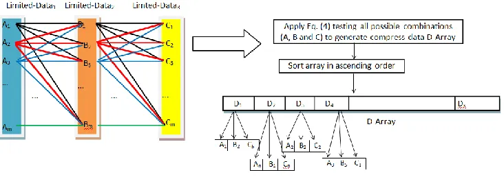
A) Initially, the Limited-Data is copied into three separated arrays given that we used three keys for compression. The algorithm picks three items of data (one from each Limited-Data) and apply these to Equation (4) using the three compression keys. The method resembles an interconnected array D,where each value is combined with each other value, similar to a network as shown in Figure7(a).

Since the three arrays of Limited-Data contain the same values, that is A1=B1=C1, A2=B2=C2 and so on the searching algorithm computes all possible combinations of A with K1, B with K2

and C with K3 that yield an intemdiate array D. As a means of an example consider that

Limited-Data1=[A1 A2 A3] , Limited-Data2=[B1 B2 B3] and Limited-Data3=[C1 C2 C3]. Then, according to Equation (4) these represent H(L), H(L+1) and H(L+2) respectively. The equation is executed 27 times (33=27) testing all possibilites. One of these combinations in array D will match the value in the compressed data. The match indicates that the unique combination of A,B and C are the original data. If we apply this to our example, Limited-Data(vertical) ={-1,0} (See

Table 1) number of possiblites for A=[-1,0], B=[-1,0] and C=[-1,0] as shown in Table 3.

Table 3: All possible data computed according to Equation (4) to generate the D-Array (K1=1,K2=3 and K3=4) Limited-Data1(A) Limited-Data2(B) Limited-Data3(C) D-Array

-1 -1 -1 -8

-1 -1 0 -4

-1 0 -1 -5

-1 0 0 -1

0 -1 -1 -7

0 -1 0 -3

0 0 -1 -4

0 0 0 0

B) The searching algorithm used in the decompression method is called Binary Search Algorithm. It finds the original data (A,B,C) for any input from compressed data file "Minimized-Array". For binary search, the D-Array should be arranged in ascending order.

sub-9

array to the right. There is no probability of “Not Matched”, because the FMS-Algorithm computes all compression data possibilities as shown in Figure-7(b).

(a) Estimate all possible compressed data saved in D-array (i.e. each possible compressed data connected with their relevent original data)

(b) Decompression by using Binary Searching algorithm

Figure 7: (a) and (b) FMS-Algorithm for reconstructing high frequency data from Limited-Data. A, B and C are the original data which are determined by the unique combination of keys.

Once the horizontal and vertical high frequency components are recovered by the FMS-Algorithm, they are combined to regenerate the 2D matrix (See Figure 6). Then each data from the matrix is multiplied by each data in Q (Equation 5) followed by the inverse DST (Equation 4) applied to each column. Finally, we multiply each data by F followed by the inverse DCT (Equation 2) applied to each row to recover the original 2D image as shown in Figure 6. If we compare the results in Figure 6 with the original 8x8 matrix of Figure 2, we find that there is not much difference, and these differences do not affect image quality. For this reason, our technique is very attractive for image compression.

6. Experimental Results

10

Additionally, we compare our compression method with JPEG and JPEG2000 through the visualization of 2D images, 3D surface reconstruction from multiple views and RMSE error measures.

Second, we apply the compression and decompression algorithms to 2D images that contain structured light patterns allowing 3D surface data to be generated from those patterns. The rationale is that a high-quality image compression is required otherwise the resulting 3D structure from the decompressed image will contain apparent dissimilarities when compared to the 3D structure obtained from the original (uncompressed) data. We report on these differences in 3D through visualization and standard measures of RMSE-root mean square error.

6.1. Results for 2D Images

In this Section, we apply the algorithms to generic 2D images, that is, images that do not contain structured light patterns as described in the previous section. In this case, the quality of the compression is performed by perceptual assessment and by the RMSE measure. We use images with varying sizes from 2.25MB to 9MB. Also, we present a comparison with JPEG and JPEG2000 highlighting the differences in compressed image sizes and the perceived quality of the compression.

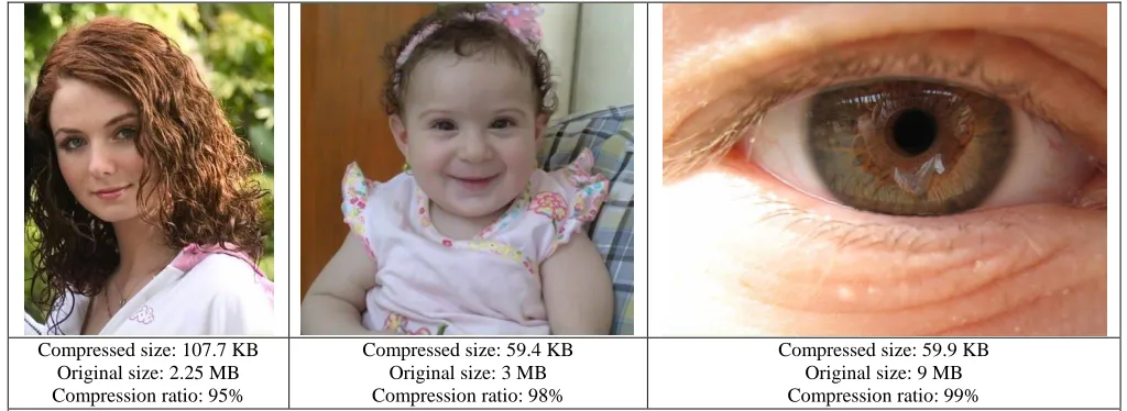
Figure 8 (a) gives an indication of compression ratios achieved with our approach while in (b) is shown details with comparative analysis with JPEG2000 and JPEG. First, the decoded 'baby' image by JPEG2000 contains some blurring at places, while the same image decoded by our approach and JPEG are of higher quality. Second, the decoded 'eyes' image by JPEG algorithm had some block artefacts resulting in a lower quality compression. Also, the same image decoded by our approach and JPEG2000 at equivalent compression ratios, has excellent image quality. Finally, the decoded 'girl' image by JPEG2000 is slightly degraded, while our approach and JPEG show good image quality.

Compressed size: 107.7 KB Original size: 2.25 MB Compression ratio: 95%

Compressed size: 59.4 KB Original size: 3 MB Compression ratio: 98%

11

Our approach: RMSE=5.95 Our approach: RMSE=4.84 Our approach: RMSE=5.94

JPEG2000: RMSE=2.71

JPEG2000: RMSE=2.83 JPEG2000: RMSE=3.49

JPEG: RMSE=3.2

JPEG: RMSE=6.66

JPEG: RMSE=5.02 (b) Details of compression/decompression by our approach,JPEG2000 and JPEG respectively

Figure 8: Compressed images by JPEG and JPEG2000 at equivalent compressed file sizes as with our approach.

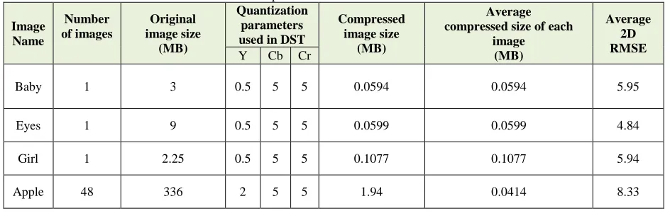
Additionally, we applied our compression techniques to a series of 2D images and used Autodesk 123DCatch software to generate a 3D model from multiple images. The objective is to perform a direct comparison between our approach and both JPEG and JPEG2000 on the ability to perform 3D reconstruction from multiple views. Images are uploaded to the Autodesk server for processing which normally takes a few minutes. The 123D Catch software uses photogrammetric techniques to measure distances between objects producing a 3D model (i.e. image processing is performed by stitching a plain seam with correct sides together). The application may ask the user to select common points on the seam that could not be determined automatically [25, 26]. Compression sizes and RMSE for all images used are depicted in Table 4.

Table 4: Compressed sizes and 2D RMSE measures

Image Name

Number of images

Original image size

(MB)

Quantization parameters used in DST

Compressed image size

(MB)

Average compressed size of each

image (MB)

Average 2D RMSE

Y Cb Cr

Baby 1 3 0.5 5 5 0.0594 0.0594 5.95

Eyes 1 9 0.5 5 5 0.0599 0.0599 4.84

Girl 1 2.25 0.5 5 5 0.1077 0.1077 5.94

12

Face 28 200.7 1 5 5 1.72 0.0629 5.68

Figure 9 shows two series of 2D images for objects “APPLE”, and “FACE” (all images are available from 123D Catch website). We start by compressing each series of images whose compressed sizes and 2D RMSE measures are shown in Table 4. A direct comparison of compression with JPEG and JPEG2000 is presented in Table 5. It is clearly shown that our approach and JPEG2000 can reach an equivalent compression ratio, while the JPEG technique does not. It is important to stress that both our technique and JPEG depend on DCT. The main difference is that our approach is based on DCT with DST and the coefficients are compressed by the frequency minimization algorithm, which renders our technique far superior to JPEG as shown in the comparative analysis of Figure 10.

Figure 9: (a) and (b) show series of 2D images used to generate 3D models by 123D Catch.

13

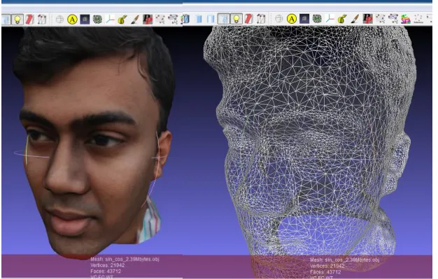
(a) 3D model for series of APPLE images decompressed by our approach (48 images, average 2D RMSE=8.33, total compressed size=1.94 MB). The compression ratio for the 3D mesh is 99.4% for connectivity and vertices

(b) 3D model for series of FACE images decompressed by our approach (28 images, average 2D RMSE=5.68, total compressed size=1.72 MB). The compression ratio for the 3D mesh is 99.1% for connectivity and vertices

Figure 10: (a) and (b) Successful 3D reconstruction following compression by our approach. Images were compressed to the same size by our approach, JPEG and JPEG2000.

Table 5: Comparison of 3D reconstruction for images compressed to the same size. Note that JPEG failed to reconstruct the 3D structure as the images were too deteriorated.

Multiple 2D images

Original size (MB)

Compressed size (MB)

2D RMSE

Our approach JPEG2000 JPEG

APPLE 336 1.94 9.5 6.58 FAIL

FACE 200.7 1.72 5.1 3.39 FAIL

6.2. Results for Structured Light Images and 3D Surfaces

14

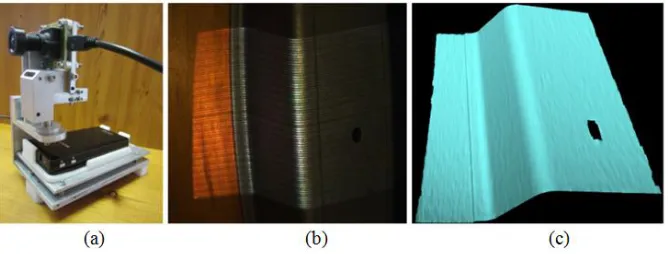
metrics in terms of error measures and perceived quality of the 3D visualization to assess the quality of the compression/decompression algorithms. The principle of operation of GMPR 3D surface scanning is to project patterns of light onto the target surface whose image is recorded by a camera. The shape of the captured pattern is combined with the spatial relationship between the light source and the camera, to determine the 3D position of the surface along the pattern. The main advantages of the method are speed and accuracy; a surface can be scanned from a single 2D image and processed into 3D surface in a few milliseconds [22]. The scanner is depicted in Figure 11.

Figure 11: (a) depicts the GMPR scanner together with an image captured by the camera (b) which is then converted into a 3D surface and visualized (c). Note that only the portions of the image that contain patterns (stripes)

can be converted into 3D; other parts of the image are ignored by the 3D reconstruction algorithms.

Figure 12 shows several test images used to generate 3D surfaces both in grayscale and colour. The top row shows two grayscale face images, FACE1 and FACE2 with size 1.37MB and dimensions 1392 ×

15

Figure 12. Structured light images used to generate 3D surfaces. Top row grayscale images FACE1 and FACE2, and colour images CORNER and METAL respectively. Images were compressed to the same size by

our approach, JPEG and JPEG2000.

Table 6: Structured light images compressed by our approach

Image Name

Original Image Size (MB)

Original Image size Compressed Size (KB)

2D RMSE 3D RMSE

DCT DST

FACE1 1.37 1 2 18.75 4.82 1.51

1 6 11.7 6.22 1.54

FACE2 1.37 1 2 15.6 1.89 2.25

1 6 7.8 2.56 2.67

CORNER 3.75 {1, 5, 5} {2, 2, 2} 21.2 5.56 1.36

{1, 5, 5} {2, 3, 3} 14.7 7.0 0.5

METAL 3.75 {1, 5, 5} {1, 5, 5} 27.5 5.25 1.87

{1, 5, 5} {2, 5, 5} 12.1 5.62 1.98

Table 6 shows the compressed size for our approach using two different values of quantization. First, the quantization scalar for FACE1 and FACE2 is 1. This means that after DCT each coefficient is divided by 1, this means rounding off each floating-point value to integer. Similarly, after DST the quantization equation is applied with F (Equation 5).

16

FACE1: Compressed size 18.75 Kbytes (texture and shaded) Compressed Size=11.7Kbytes (shaded) 3D reconstructed FACE1 from decompressed image by our approach

FACE2: Compressed size 15.6 Kbytes (texture and shaded) Compressed Size=7.8 Kbytes (shaded) 3D reconstructed FACE2 from decompressed image by our approach

2D decompressed images zoomed-in, to show the details: FACE1 and FACE2 at higher compression ratio

Figure 13: Top: FACE1 shows decompressed 3D surface with texture and shaded at compressed size 18.7KB and 11.7KB. Middle: FACE2 shows decompressed 3D surface with texture and shaded at compressed size 15.6KB and

7.8KB. Bottom: details of 2D images FACE1 and FACE2 respectively at the higher compression ratio.

17

CORNER: Compressed size 21.2 Kbytes (texture and shaded) Compressed Size=14.7 Kbytes (shaded)

3D reconstructed CORNER from decompressed image by our approach

METAL: Compressed size 27.5 Kbytes (texture and shaded) Compressed Size=12.1 Kbytes (shaded)

3D reconstructed METAL from decompressed image by our approach

2D decompressed images zoomed-in, to show the details: CORNER and METAL at higher compression ratio

Figure 14: (Top) shows decompressed 3D surface of CORNER with texture and shaded at compressed sizes 21.2KBand 14.7KB. (Middle) shows decompressed 3D surface of METAL with texture and shaded at compressed sizes 27.5KB and 12.1KB. (Bottom) zoomed-in details for 2D images CORNER and METAL respectively at higher compression ratio.

18

JPEG2000 - 18.75 Kbytes JPEG2000 - 11.7 Kbytes JPEG2000 - 15.6 Kbytes JPEG2000 - 7.8 Kbytes

JPEG2000 - 21.2 Kbytes JPEG2000 - 14.7 Kbytes

Figure 15: Top: 3D reconstructed surface for FACE1 and FACE2 respectively using JPEG2000. Bottom: CORNER image successfully 3D reconstructed, while METAL image failed 3D reconstruction.

Table 7: Compression and decompression for 3D reconstruction by JPEG2000 and JPEG at higher compression ratios. All images were compressed to the same size by the techniques.

Image name

Compressed Size (KB)

JPEG2000 JPEG

2D RMSE

3D RMSE

2D RMSE

3D RMSE

FACE1 11.7 6.3 1.8 FAIL FAIL

FACE2 7.8 3.2 2.66 FAIL FAIL

CORNER 14.7 5.7 0.63 FAIL FAIL

METAL 13.4 4.17 FAIL FAIL FAIL

19

does, the 3D surface contains some degradation. Additionally, Figure 16 shows the compressed 2D images by JPEG2000 with zoomed in image details.

Figure16: Details of 2D decompressed images by JPEG2000: Top: FACE1 on the left is clearly blurred leading to degraded 3D reconstruction. Bottom: METAL image on the right is blurred rendering it unable to reconstruct

a 3D surface.

7. Conclusions

20

The most important aspects of the method and their role in providing high quality image with high compression ratios are identified as follows:

1. The one-dimensional DCT can be applied to an image row (i.e. larger block sizes ≥ 8). Equally, the one-dimensional DST can be applied to each column of the output from DCT.

2. The user can ignore the scalar quantization to remove higher frequency coefficients (i.e. keeping more coefficients increases image quality).

3. The two-dimensional quantization (cf. Equation 5) provides a more aggressive quantization removing most of matrix contents as about 50% of the matrix entries are zero. Applying this over the DST can keep image quality at higher compression ratios.

4. The final transformed matrix is divided into: low-frequency sub-matrix, and horizontal and vertical high-frequency matrices.

5. The minimization of high frequency algorithm produces a Minimized-Array used to replace each three values from the high-frequencies sub-bands by a single integer value. This process reduces the coefficients by 2/3 leading to increased compression ratios.

6. Since the Minimized-Array for both vertical and horizontal high-frequencies contains large number of zeros, we applied a new method to eliminate zeros and keep nonzero data. The process keeps significant information while reducing data up to 80%.

7. At decompression stage, the Fast-Matching-Search algorithm is the engine for estimating the original data from the minimized array and depends on the organized key values and the availability of a set of unique data. The efficient C++ implementation allows this algorithm to recover the high-frequency matrices very efficiently.

8. The key values and unique data are used for coding and decoding an image, without this information images cannot be recovered. This is an important point as a compressed image is equivalent to an encrypted image that can only be reconstructed if the keys are available. This has applications to secure transmission and storage of images and video data.

9. Our proposed image compression algorithm was tested on true colour and YCbCr layered images at high compression ratios. Additionally, the approach was tested on images resulting in better 3D reconstruction than JPEG2000 and JPEG.

10. The experiments indicate that the technique can be used for real-time applications such as 3D data objects and video data streaming over the Internet.

Future work is focused on efficient implementation of the decoding steps and their application to video compression. Research is underway and will be reported soon.

References

[1] A. Al-Haj, (2007) Combined DWT-DCT Digital Image Watermarking, Science Publications, Journal of Computer Science 3 (9): 740-746.

[2] C. Christopoulos, J. Askelof, andM. Larsson (2000) Efficient methods for encoding regions of interest in the upcoming JPEG 2000 still image coding standard, IEEE Signal Processing Letters,vol.7,no.9.

[3] S. A. Martucci, Symmetric convolution and the discrete sine and cosine transforms, IEEE Trans. Sig. Processing SP-42, 1038-1051 (1994).

[4] I.E. G. Richardson (2002) Video Codec Design, John Wiley &Sons.

[5] K. Sayood, (2000) Introduction to Data Compression, 2nd edition, Academic Press, Morgan Kaufman Publishers.

[6] Pennebaker, William B., and Joan L. Mitchell, JPEG: Still Image Data Compression Standard, Van Nostrand Reinhold,

21

[7] H. B. Kekre, TanujaSarodeandPrachiNatu (2013), EFFICIENT IMAGE COMPRESSION TECHNIQUE USING FULL,

COLUMN AND ROW TRANSFORMS ON COLOUR IMAGE, International Journal of Advances in Engineering &

Technology, Vol. 6, Issue 1, pp. 88-100

[8] EvaldoGonqalvesPelaesandYuzolano (1998), IMAGE CODING USING DISCRETE SINE TRANSFORM WITH AXIS

ROTATION, IEEE Transactions on Consumer Electronics, Vol. 44, No. 4, pp 1284-1290

[9] Discrete Sine Transform (2016) https://en.wikipedia.org/wiki/Discrete_sine_transform, last accessed Nov. 2016

[10]Swati DhamijaandDr. Priyanka Jain (2011),Comparative Analysis for Discrete Sine Transform as a suitable method for noise estimation, IJCSI International Journal of Computer Science Issues, Vol. 8, Issue 5, No 3, September 2011

[11]Malini. S and Moni. R. S (2014), Use of Discrete Sine Transform for A Novel Image Denoising Technique, International Journal of Image Processing (IJIP), Volume (8) Issue (4) 2014

[12] Knuth, Donald (1997). Sorting and Searching: Section 6.2.1: Searching an Ordered Table, The Art of Computer Programming 3 (3rd Ed.), Addison-Wesley. pp. 409–426. ISBN 0-201-89685-0

[13]M. Rodrigues, A. Robinson and A. Osman, (2010) Efficient 3D data compression through parameterization of free-form surface patches, In: Signal Process and Multimedia Applications (SIGMAP), Proceedings of the 2010 International Conference on. IEEE, 130-135.

[14]M.M. Siddeqand G. Al-Khafaji, (2013) Applied Minimize-Matrix-Size Algorithm on the Transformed images by DCT and DWT used for image Compression, International Journal of Computer Applications, Vol.70, No. 15.

[15]M.M. Siddeq and M.A. Rodrigues, (2014a) A New 2D Image Compression Technique for 3D Surface Reconstruction,

18th International Conference on Circuits, Systems, Communications and Computers, Santorin Island, Greece: 379-386 [16]M.M. Siddeqand M.A. Rodrigues(2014b) A Novel Image Compression Algorithm for high resolution 3D Reconstruction,

3D Research. Springer Vol. 5 No.2.DOI 10.1007/s13319-014-0007-6

[17]M.M. Siddeqand RODRIGUES, Marcos (2015a). Applied sequential-search algorithm for compression-encryption of high-resolution structured light 3D data. In: BLASHKI, Katherine and XIAO, Yingcai, (eds.)MCCSIS : Multi-conference on Computer Science and Information Systems 2015. IADIS Press, 195-202

[18]M.M. Siddeq and RODRIGUES, Marcos (2015b). A novel 2D image compression algorithm based on two levels DWT and DCT transforms with enhanced minimize-matrix-size algorithm for high resolution structured light 3D surface reconstruction. 3D Research, 6 (3), p. 26. DOI 10.1007/s13319-015-0055-6

[19]M. Rodrigues, A. Osman and A. Robinson, (2013a) Partial differential equations for 3D data compression and reconstruction, Journal Advances in Dynamical Systems and Applications.12(3), 2004, pp 371–378

[20]M. Rodrigues, M. Kormann, C. Schuhlerand P. Tomek(2013b) Robot trajectory planning using OLP and structured light 3D machine vision. Lecture notes in Computer Science Part II. LCNS, 8034 (8034). Springer, Heidelberg, 244-253. [21]M. Rodrigues, M. Kormann, C. Schuhlerand P. Tomek (2013c). Structured light techniques for 3D surface

reconstruction in robotic tasks. In: KACPRZYK, J, (ed.) Advances in Intelligent Systems and Computing. Heidelberg, Springer, 805-814.

[22]M. Rodrigues, M. Kormann, C. Schuhlerand P. Tomek (2013d). An intelligent real time 3D vision system for robotic welding tasks. In: Mechatronics and its applications. IEEE Xplore, 1-6.

[23]R. C. Gonzalez and R. E. Woods (2001) Digital Image Processing, AddisonWesleypublishing company.

[24]T. Acharya and P. S. Tsai. (2005) JPEG2000 Standard for Image Compression: Concepts, Algorithms and VLSI Architectures. New York: John Wiley & Sons.

[25]Autodesk 123D,https://en.wikipedia.org/wiki/Autodesk_123D, last accessed May-2016