Forecasting Volatility in Developing Countries' Nominal Exchange Returns

Munich Personal RePEc Archive

Forecasting Volatility in Developing

Countries’ Nominal Exchange Returns

Antonakakis, Nikolaos and Darby, Julia

Vienna University of Economics and Business, Department of

Economics, University of Strathclyde

26 August 2012

1

FORECASTING VOLATILITY IN DEVELOPING COUNTRIES’

NOMINAL EXCHANGE RETURNS

Nikolaos Antonakakis (Corresponding author) Department of Economics Institute for International Economics Vienna University of Economics and Business

Althanstrasse 39-45, Vienna, Austira Tel.: +43/1/313 36-4141 Email: [email protected]

Julia Darby Department of Economics

University of Strathclyde 130 Rottenrow, Glasgow, G4 0GE

Tel:

+44 (0)141 548 3859

August 26, 2012

Abstract

This paper identifies the best models for forecasting the volatility of daily exchange returns of developing countries. An emerging consensus in the recent literature focusing on industrialised counties has noted the superior performance of the FIGARCH model in the case of industrialised countries, a result that is reaffirmed here. However, we show that when dealing with developing countries’ data the IGARCH model results in substantial gains in terms of the in-sample results and out-of-sample forecasting performance.

Keywords: Exchange rate volatility, estimation, forecasting, developing countries

2

1. Introduction

Developing countries are increasingly being regarded as alternative destinations for foreign investment flows (WIPS, 2010). This change has been accompanied by a huge increase in international transfers, and in many cases by unexpected changes in exchange rate volatility. Such changes can be very costly for investors if they are unforeseen or inefficiently managed. A key question this paper seeks to address is whether the same volatility models that have been used widely and successfully in previous studies of industrialised countries’ exchange rate volatility perform equally well in terms of in-sample and out-of-sample performance when applied to data for developing countries.

There may be good reasons to expect models to perform differently with developing vs industrialised country data. For example, management of risks associated with unexpected changes in exchange rate volatility can be facilitated through access to forward contracts and/or other hedging instruments, but these are less widely available for developing countries. The country groups also differ in terms of their historical experiences of financial crises. The existing empirical literature on forecasting daily exchange rate volatility in industrialised countries is extensive but that using data from developing countries is relatively sparse, although the gains to achieving a greater understanding of volatility in this setting are potentially large.1 This paper tries to address this gap. We consider various well established conditional heteroskedasticity models and assess both their within sample fit and out-of-sample forecasting performance.

Our motivation to focus on the forecasting performance of various exchange rate volatility models in developing versus industrialised countries for daily data in part derives from the fact that a number of studies document far greater exchange rate volatility in developing as opposed to industrialised countries. For example, Devereux and Lane (2003) analysed an extensive sample of 158 countries (23 industrialised and 135 developing country bilateral exchange rates with the US dollar over the period 1995-2000). Theyfound that monthly exchange rate volatility in developing countries, as measured by the standard deviation of the first differences in logged bilateral exchange rate, was almost 2.5 times greater than that in industrialised countries. Using a similar framework, Hausmann et.

1

3

al. (2006) found that exchange rate volatility in developing countries was approximately three times greater than that in industrialised countries (they looked at real effective exchange rates and they applied panel techniques to data for 74 industrialised and developing countries over the period 1980-2000 at an annual frequency). They determined that this difference in volatility could not be explained by: i) the fact that developing countries are more likely to face larger macroeconomic shocks (e.g. to their terms of trade, GDP growth and inflation); ii) their greater likelihood of experiencing recurrent currency crises; or iii) by a higher elasticity of exchange rate volatility with respect to these shocks. In contrast, and through employing (G)ARCH models, they were able to provide evidence that the difference in exchange rate volatility experienced by developing and industrialised countries could in part be explained by differing persistence of the exchange rate volatility itself. This finding suggests that using models capable of capturing differential persistence of exchange rate volatility are likely to be of particular relevance to our endeavour.

A common feature of the two studies mentioned above, and many others, is the use of low frequency, i.e. monthly or annual data, rather than higher frequency daily or intra-daily data. Often the use of low frequency data reflects the fact that the authors were aiming to evaluate the extent to which exchange rate volatility can be explained by macroeconomic variables such as gross domestic product, inflation and exports. These macroeconomic variables are typically only available at a relatively low frequency, monthly at best, and more often quarterly or annual. In contrast it has been argued that many of the drivers of dynamics in exchange rate returns and volatility, including microstructure effects, can best be identified in high-frequency data (see, for instance, Andersen and Bollerslev, 1998a, Andersen and Bollerslev, 1998b, Andersen et al., 1999, 2001 and 2003). In this paper we are interested in capturing daily exchange rate volatility dynamics, and do not focus on explaining longer horizon volatility in the developing countries, which we leave for further research.

4

The remainder of the paper is organized as follows. Section 2 describes the data and methodology employed. Section 3 presents the empirical results of the in-sample estimation and out-of-sample performance and section 4 concludes.

2. Data and Methodology

The data used here consist of daily observations on four spot exchange rates against the US dollar obtained from Oanda database2,3. The exchange rates under consideration are: the Botswana pula (BWP), Chilean peso (CLP), Cyprus pound (CYP) and Mauritius rupee (MUR). The choice of these four specific countries was based on the fulfilment of the following criteria: i) that they were included among that developing countries in Devereux and Lane (2003); ii) that have not fixed their currency with the US dollar4,our base currency, during our sample period;and iii) that daily spot exchange rate data is available. After careful inspection, the developing countries that fulfilled these conditions were the four mentioned above. Our in-sample estimation period runs from 8/11/1993 to 29/12/2000, totalling 1806 observations. The choice of the sample was chosen for the ease of comparison with earlier studies we refer to that forecast exchange rate volatility in industrialised countries. Weekends, Christmas, Easter and bank holidays are excluded from the sample, since during these periods transactions are nonexistent or so limited that their inclusion could distort the estimation results.

Results are presented for six alternative conditional heteroskedasticity models. Specifically we considered ARCH, GARCH, EGARCH, IGARCH, FIGARCH and the HYGARCH models. Given that there is no guidance in the literature on exchange rate volatility forecasting in developing countries on selecting the "best" model, we began our analysis with a simple ARCH model and progressively extended the analysis to more sophisticated models.

2

Ultimately would be preferable to use intra-daily data but since exchange rate data in developing countries were only available to us on a daily basis, we focus on daily data for this group of countries.

3

We have also collected daily data from the same database for our control group of industrialised countries consisting of the British pound (GBP), Swiss franc (CHF), Japanese yen (JPY) and the Norwegian Krone (NOK).

4

5

The Autoregressive Conditional Heteroskedasticity (ARCH) model of Engle’s (1982) estimates the conditional variance of a time series 𝑦𝑡,𝑉𝑎𝑟(𝑦𝑡|𝑦𝑡−1) = 𝜎𝑡2as an autoregressive (AR) process which can be written as:

𝜎𝑡2=𝛿+𝛼1𝜀𝑡−12 +𝛼2𝜀𝑡−22 +⋯+𝛼𝑞𝜀𝑡−𝑞2 +𝜔𝑡 =𝛿+𝛼(𝐿)𝜀𝑡−12 +𝜔𝑡 (1)

where 𝜔_𝑡 is a white noise and 𝛼(𝐿) is a lag polynomial of order 𝑞 −1. One restriction that must be fulfilled in order for the model to be readily interpretable is that the conditional variance is positive. To ensure that the conditional variance is positive, 𝛿 must be positive and the coefficients in 𝛼(𝐿)

must be greater than, or equal to, zero. In addition, to ensure that the process is stationary, 𝛼(𝑞) must be strictly less than unity. If the coefficients 𝛼𝑖 are positive, and if recent squared errors are large, the ARCH model predicts that the current squared errors will be large in magnitude, in the sense that its variance 𝜎_𝑡2 is large.

Bollerslev (1986) extended the ARCH model to allow the error variance to depend on its own lags as well as lags of the squared error. In other words, his extension allows the conditional variance to follow an Auto Regressive Moving Average (ARMA) process, which can be specified as:

𝜎𝑡2=𝛿+𝛼1𝜀𝑡−12 +⋯+𝛼𝑞𝜀𝑡−𝑞2 +𝛽1𝜎𝑡−12 +⋯+𝛽𝑝𝜎𝑡−𝑝2 +𝜔𝑡

= 𝛿+� 𝛼_𝑖𝜀_𝑡−𝑖2

𝑞

𝑖=1

+� 𝛽_𝑗𝜎_𝑡−𝑗2

𝑝

𝑗=1

=𝛿+𝛼(𝐿)𝜀_𝑡−12 +𝛽(𝐿)𝜎_𝑡−12 +𝜔_𝑡

(2)

where 𝛼(𝐿) =𝛼1𝐿+𝛼2𝐿2+⋯+𝛼𝑞𝐿𝑞 and 𝛽(𝐿) =𝛽1𝐿+𝛽2𝐿2+⋯+𝛽𝑝𝐿𝑝 are lag polynomials. According to Engle and Bollerslev (1986) if we define the surprise in the squared innovations as

𝑢𝑡 ≡ 𝜀𝑡2− 𝜎𝑡2 then the GARCH(1,1) process can be rewritten as:

6

i.e. the squared errors follow an ARMA(1,1) process, so while the error 𝑢𝑡 is uncorrelated over time, it does exhibit heteroskedasticity. Furthermore, the root of the autoregressive part is 𝛼+𝑏, so stationarity requires that𝛼+𝑏< 1. The GARCH(p,q) process can be defined by:

𝜎𝑡2=𝛿+� 𝛼𝑖𝜀𝑡−𝑖2 𝑞

𝑖=1

+� 𝛽𝑗𝜎_𝑡−𝑗2

𝑝

𝑗=1 (4)

where the conditional variance is a linear function of a constant, 𝑞 lags of the past squared error terms and 𝑝 lags of the past squared conditional variances. The necessary conditions needed to ensure that the conditional variance 𝜎_𝑡2 is strictly positive are the following: 𝛿> 0, 𝛼𝑖 ≥0, 𝛽_𝑗≥0, 𝑖= 1,2, … ,𝑞, 𝑗= 1,2, … ,𝑝. The weak stationarity of this model is assured by:

� 𝛼𝑖 𝑞

𝑖=1

+� 𝛽_𝑗

𝑝

𝑗=1

< 1.

(5)

The GARCH(1,1) model, in general terms, performs well in terms of tracking short-run dependencies in volatility and explaining the characteristics of the financial times series such as exchange rate returns series (Hansen and Lunde, 2005).

Another extension of the GARCH model employed in this study is the Exponential GARCH (EGARCH) model introduced by Nelson (1991). The EGARCH model allows for an asymmetric response to a shock, meaning that good news has a different impact to bad news on volatility. The EGARCH can be defined by:

𝑙𝑜𝑔𝜎𝑡2=𝜔+ [1− 𝛽(𝐿)]−1[1 +𝛼(𝐿)]𝑔(𝑧𝑡−1) (6)

7

function of both the magnitude and the sign of 𝑧𝑡”. For that reason the author defines the function

𝑔(𝑧𝑡) by:

𝑔(𝑧𝑡) = 𝜃1𝑧𝑡_�

𝑠𝑖𝑔𝑛𝑒𝑓𝑓𝑒𝑐𝑡

+𝜃2_{�����������}[|𝑧𝑡|− 𝐸|𝑧𝑡|]

𝑚𝑎𝑔𝑛𝑖𝑡𝑢𝑑𝑒𝑒𝑓𝑓𝑒𝑐𝑡

, (7)

Because the level 𝑧_𝑡 is included, the EGARCH model is asymmetric as long as 𝜃₁≠0. When 𝜃₁< 0, positive shocks (‘good news’) generate less volatility than negative shocks (‘bad news’). When 𝜃₁> 0, negative shocks (‘bad news’) generate less volatility than positive shocks (‘good news’).

As noted above, many studies that have examined daily exchange rate data for industrialised countries have reached the conclusion that volatility is highly persistent and tends to be well approximated by an IGARCH process (see e.g., Bollerslev 1987, McCurdy and Morgan 1988, Baillie and Bollerslev 1989, and Hsieh 1989). Nevertheless, the extremes offered by the exponential decay assumed in the GARCH model and infinite persistence assumed in the IGARCH model might be overly restrictive. If the dispersion of shocks to the conditional variance decays at a slow hyperbolic rate, then, a more flexible class of processes can be adopted, and should be more capable of capturing the long run dependencies in observed exchange rate volatility. On this basis we consider the Fractionally Integrated Generalized Autoregressive Conditionally Heteroskedastic (FIGARCH) model introduced by Baillie, Bollerslev and Mikkelsen (1996). The FIGARCH model incorporates a lag polynomial term of the form (1− 𝐿)𝑑, for non-integer 𝑑, and thereby allows a long memory process in the conditional variance. If the actual autocorrelations in conditional variance decay at a hyperbolic rate, this model is expected to perform relatively well at longer horizons. The FIGARCH extends the GARCH model by allowing a term of the form (1− 𝐿)𝑑, defined by:

�1− 𝜑(𝐿)�(1− 𝐿)𝑑𝜀_𝑡2=𝜔+�1− 𝛽(𝐿)�(𝜀_𝑡2− 𝜎_𝑡2)

or

𝜎𝑡2=𝜔∗+ {1−[1− 𝛽(𝐿)]−1𝜑(𝐿)(1− 𝐿)𝑑}𝜀𝑡2

(8.a)

8

where the constant is now defined as 𝜔∗ =𝜔[1− 𝛽(𝐿)]−1 and 𝑑 ∈(0,1).

Davidson (2004) proposed a generalized version of the FIGARCH model the Hyperbolic GARCH (HYGARCH) model. This model can generate long memory without ‘behaving oddly’ when d, the parameter of fractional integration, approaches 1. The HYGARCH model is given by the following equation:

2

_[1

_{( )]}

_{{1 [1}

_{( )}

_{( ){1}

_[(1

_{) ]}}}

t

L

L

L

L

σ

₌

ω

₋

β

_{+ − −}

β

φ

₊

α

₋

ε

(9)

Interestingly, the HYGARCH nests the FIGARCH when𝛼= 1, or equivantly when log(𝛼) = 0, and the process is stationary when𝛼< 1, or equivantly when log(𝛼) < 0, in which case the GARCH component observes the usual covariance stationarity restrictions (see Davidson, 2004).5

The criterion for model selection across each of the six GARCH-type models is based on in-sample and out-of-in-sample diagnostic tests. The in-in-sample diagnostics include the Akaike Information Criterion (AIC), Schwarz Bayesian Criterion (SBC), Hannan-Quinn Criterion (HQC), Shibata Criterion (SC), log-likelihood values, Box-Pierce statistics on both raw (𝑄) and squared (𝑄2) standardized residuals and Engle’s LM ARCH test for the presence of further ARCH effects. Under the Student-t or Skewed-Student-t distribution, the model with the minimum AIC, SBC, HQC, SC, maximum log-likelihood values and which passes the Q-, Q-squared and the LM ARCH test simultaneously is adopted. In each case a choice has to be made on the appropriate number of lags of the squared errors to include in each of the equation. We referred to residual based tests and information criteria, specifically AIC (Akaike Information Criteria), SBC (Schwarz Bayesian Criteria) and HQC (Hannan-Quinn Criteria). In the case of out-of-sample selection, the model with the smallest forecast error of the various tests is adopted.

The covariance matrix of the estimates is computed using a Quasi-Maximum Likelihood (QML) method. In addition, the optimization method of the QML procedure is done primarily under

5

9

the standard QML approach that uses the quasi-Newton method of Broyden, Fletcher, Goldfarb and Shanno (BFGS). However, in cases where this conventional BFGS optimization algorithm fails to converge, we turn to an alternative, the Simulated Annealing (SA) algorithm proposed by Goffe, Ferrier and Rogers (1994). Some of the problems that the BFGS algorithm may encounter during estimation are summarised in Cramer (1986, p. 77) are: i) the algorithm may not converge in a reasonable number of steps, ii) it may head toward infinitely large parameter values, or even loop through the same point time and again and iii) it may have difficulty with ridges and plateaus. When faced with such difficulties, the researcher might be able to overcome them through use of different starting values. However, Goffe, Ferrier and Rogers (1994, p. 66) state that “even if the algorithm converges, there is no guarantee that it will have converged to a global, rather than a local, optimum since conventional algorithms cannot distinguish between the two”. The key advantages of the algorithm proposed by Goffe, Ferrier and Rogers (1994) are that it is less dependent on the specific starting values used6 and can focus in on global rather than local optima by exploring the relevant function’s entire surface and moving both uphill and downhill.

For the first five models we assess parameter significance by making use of the Student-t Distribution. In the case of the HYGARCH model our inference is based on the skewed-Student-t Distribution, as recommended in Davidson (2004).7 Both the Student-t and the skewed-Student-t distributions take into account the phenomenon of greater leptokurtosis and skewness in the probability density function as compared to the normal distribution.

In terms of forecasting performance, 253 observations ranging from 2/01/2001 to 31/12/2001 are used for out-of-sample forecast evaluation. The 253 out-of-sample volatility forecasts are produced for the one-step ahead daily forecast horizon. In order to produce 253 daily volatility forecasts the equations are estimated 253 times and estimated recursively. The accuracy of exchange rate volatility forecasts is evaluated through reference to the most commonly used criteria. These include a Mincer

6

The SA algorithm was applied only if there is no convergence under the conventional BFGS algorithm. In our research, since no convergence was obtained in the case of the developing countries, the SA algorithm was used throughout.

7

10

and Zarnowitz’s (1969) regression based test, the Mean Square Forecast Error (MSFE) and the Superior Predictive Abilitity (SPA) test developed by Hansen (2005). In the case of the Mincer and Zarnowitz (1969) regression based test, the true (or realized) volatilityis regressed on a constant and forecast volatility for each model:

𝜎𝑠𝑞𝑢𝑎𝑟𝑒𝑑𝑟𝑒𝑡𝑢𝑟𝑛𝑠,𝑡+1 =𝛼+𝛽𝜎�𝑓𝑜𝑟𝑒𝑐𝑎𝑠𝑡,𝑡+1+𝜀𝑡 (10)

For a given model’s forecast to be unbiased, the parameters 𝛼 and 𝛽 from equation (10) should be take the values 0 and 1 respectively. We test whether these theoretical restrictions are data admissible. In addition, the 𝑅2 (goodness-of-fit) of this regression is used as a measurement of predictive power of the various models considered. The model that achieves the largest 𝑅2 is the one for which the forecast best approximates true volatility, so has the most powerful forecasting ability. True volatility is proxied by the daily squared ex-post returns. This approach has been widely used in exchange rate volatility forecasting evaluation (see, for instance, Anderson and Bollerslev 1998a; Balaban, 2004; Martens, Chang and Taylor, 2002 and Pong, Shackleton, Taylor and Xu, 2004).

The second and most widely used accuracy measures in volatility forecasting literature is the MSFE. The MSFE for a sample size 𝑇 is a quadratic loss function and defined by:

𝑀𝑆𝐹𝐸 =1

𝑇 � 𝑒𝑡+12 ,𝑡

𝑇

𝑡=1

(11)

11

the minimum MSFE is preferred. This criterion has been widely and successfully used in many studies of exchange rate volatility forecasting (see, for instance, Vilasuso, 2002 and Balaban, 2004).8

A key feature of out-of sample criteria, including the MSFE, is that the model with the smallest forecast error is preferred. However, it is useful to know whether the model with the smallest forecast error is significantly superior to the other models or not – it may be worth trading off a slightly larger forecast error for a simpler model, if the difference in forecasting performance is insignificant. In order to be able to evaluate whether one model forecasts significantly better than another we look at an equal accuracy test proposed by Diebold and Mariano (1995). The DM tests need to be conducted on pairwise comparisons of models, while in practice the interest of the researcher is often to choose between models m models (where 𝑚> 2). For this reason, our preferred test is the Superior Predictive Ability (SPA) test proposed by Hansen (2005) which permits evaluation of the performance of all alternative models simultaneously. The SPA test evaluates whether the same outcomes can be achieved by more than one model and uses a bootstrap procedure. Specifically, a target model is selected by one of the evaluation criteria and the question of interest is whether any of the alternative forecasts are better, according to a pre-determined loss function, than the target forecast. Following Hansen9, the chosen loss function is based on MSFE.

3. Empirical Results

3.1. Descriptive Statistics

Table 1 provides the summary statistics of exchange rate returns for each of the four currencies against the US dollar in developing countries, respectively. Exchange returns are calculated as the first difference in the natural logarithm of the nominal exchange rate.

[Insert Table 1 here]

8

Patton (2011) derives necessary and sufficient conditions on the functional form of the loss for the ranking of volatility forecasts to be robust to the presence of noise in the volatility proxy. He also shows that the MSFE loss is robust.

9

12

As indicated in Table 1, the series all show evidence of significant excess kurtosis10. This indicates that daily exchange rate returns are heavy-tailed (leptokurtic) so tend to contain more extreme values than would be expected under the normal distribution. Another feature of the data that is picked up in Table 1 is significant positive skewness. Positive skewness is indicative greater prevalence of depreciations as opposed to appreciations in the developing countries in our sample. Consistent with the results on skewness and kurtosis, the Jarque-Bera normality test strongly rejects the null hypothesis that returns are normally distributed. Inference is therefore based on Student-t or Skewed-Student-t distribution which is have been shown to perform better in these circumstances (see, for instance, Bollerslev, 1987; Hsieh, 1989; and Baillie and Bollerslev, 1989, among others).

Aside from the results for the CYP/USD, Table 1 offers strong evidence of ARCH effects in the exchange rate returns series. Formally, using the ARCH LM test we reject the null hypothesis of no ARCH effect in the residuals, similarly there is evidence of significant serial correlation in the standardised squared returns on the basis of the Ljung-Box Q statistics at every lag tested. In the case of CYP/USD, while we cannot reject the null hypothesis of ARCH effects, the Ljung-Box statistic offers evidence of serial correlation in the standardized squared returns at up to 20 lags, suggesting that there is evidence of higher order dependence.

3.2. Estimation results

In this section we present the in-sample estimation results for the ARCH, GARCH, EGARCH, IGARCH, FIGARCH and HYGARCH models.

The conditional mean and variance specifications were initially estimated under the conventional BFGS algorithm but the algorithm failed to achieve convergence. This finding is consistent with Cramer (1986, p.77). Once we switched to using the Simulated Annealing (SA) algorithm of Goffe, Ferrier and Rogers (1994) we were able to achieve convergence to a global

10

The excess kurtosis is defined as: 𝐾=𝐸[(𝑦−𝜇)4]

𝜎4 −3. A distribution with positive excess kurtosis is said to

13

maximum11. The in-sample estimation results and the residual diagnostics for the six conditional volatility models of the Chilean peso (CLP), Cyprus pound (CYP), Botswana pula (BWP) and the Mauritian rupee (MUR) exchange returns are presented in Tables 2, 3, 4 and 5, respectively. The conditional mean of each exchange rate return series was modelled as an autoregressive process of order 1 or AR(1).

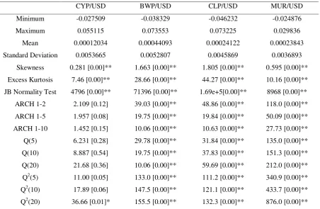
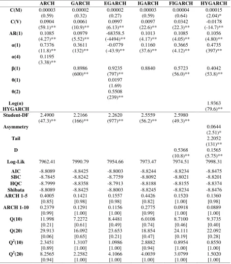
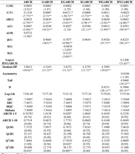
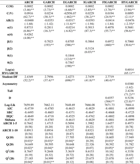
The results of the ARCH model are shown for comparison but can easily be improved upon in all cases. In all but the CYP/USD case the stationarity constraint is not met as α(q)>1, and in most cases (all but CLP/USD) evidence of higher order serial correlation in the squared standardized residuals cannot be rejected at the 5% level of significance. Furthermore comparing across models, the GARCH, IGARCH, FIGARCH and HYGARCH models all achieve lower values of the information criteria. A GARCH (1,1) model, shown in the second column of Tables 2 through 5, seems better able to capture the time varying volatility in all four exchange returns series. In each case the key parameters are significant at the 5% level of significance. In addition, the positivity and stationarity constraints are met as 𝛼�₁+𝛽̂₁ ≥0 and 𝛼�₁+𝛽̂₁< 1, with the exception of the CLP/USD model where

𝛼�1+𝛽̂1> 1. In each case however, the sum of 𝛼�1+𝛽̂1 is very close to one and a sum of unity could

not be rejected on the basis of an LR test. This evidence of strong persistence suggests that the series may be better approximated in a specification that captures a wider range of long run dependencies.

Prior to analysing the processes that account for long run dependencies, we check for asymmetric responses to good and bad shocks using the EGARCH specification, the results are presented on column three of Tables 2 through 5. The key estimated parameter here is 𝜃�₁ in Equation (7) and is positive but insignificant at the 5% level for the CLP/USD and MUR/USD return series, significantly positive at 5% for the BWP/USD and significantly negative at 5% for the CYP/USD return series. A significant and positive 𝜃�1 means that positive shocks (‘good news’) generate more volatility than negative shocks (‘bad news’) for the case of BWP/USD, and vice versa for a significant

11

14

negative 𝜃�₁ in the case of the CYP/USD return series. However, problems with this specification are evident in the estimated 𝛼�₁, and in the case of BWP/USD the positivity constraint is not ensured.

[Insert Tables 2-5 here]

In addition, the residual diagnostics for the CYP/USD and BWP/USD series provide evidence that significant higher order serial correlation remains in squared standardized residuals remains, so not all the conditional heteroscedasticity evident in the data is captured by the model. While asymmetries of this kind have been supported in research by Balaban (2004), Bollerslev, Chou and Kroner (1992) and Kisinbay (2010), our evidence suggests that the EGARCH formulation is not appropriate in capturing the time varying volatility for all four developing countries’ exchange rate return series12.

Our analysis continues with estimation of the IGARCH model for each of the four exchange return series, results are presented on the fourth column of Tables 2 through 5. In all four exchange returns series the estimated parameters are significant at 5%. In addition, the residual diagnostics indicate that there is no evidence of remaining ARCH effects and no serial correlation for the standardized and squared standardized residuals. The IGARCH model appears to fits well the CLP/USD, CYP/USD, BWP/USD and MUR/USD exchange return series.

The next model under investigation which accounts for long run dependencies in volatility is the FIGARCH model. The parameter estimates and the residuals tests of the FIGARCH models are presented on the fifth column of Tables 2 through 5. The long memory parameter d captures decay in the memory of a shock to the conditional variance. In each case 𝑑̂ is significant at the 1% level. Moreover, the rest of the parameters of the FIGARCH model are also significant. However, the residual diagnostics are not entirely satisfactory. In the case of the BWP/USD return series there is evidence of up to 20th order serial correlation in the standardized residuals. In the case of the MUR/USD return series there is evidence of 20th order serial correlation in the standardized residuals

12

15

and up to 20th order serial correlation in the squared standardized residuals. In these cases the diagnostics for the IGARCH specification are preferable.

The final model under investigation is the HYGARCH model. The estimated parameters and the residual diagnostics are presented in the last column of Tables 2 through 5. All the estimated parameters of the HYGARCH model are significant but the estimated parameter log(𝛼�) in all four cases is greater than zero. This means that the HYGARCH process does not satisfy the stationary condition: log(𝛼�) < 0. We therefore conclude that the HYGARCH model is not appropriate in these cases.

In conclusion, among these six volatility models, the GARCH the IGARCH and the FIGARCH models seem to perform better than the ARCH, EGARCH and the HYGARCH models in terms of capturing the time varying volatility in developing countries’ exchange return series. Among the GARCH, IGARCH and the FIGARCH models, although the FIGARCH model has the highest log-likelihood values, the information criteria (specifically the AIC, SBC, HQC and Shibata) are minimised for the IGARCH model in the case of the CYP/USD and MUR/USD return series. For the CLP/USD and BWP/USD series the information criteria are minimised for the GARCH and the FIGARCH model respectively. However, the GARCH model in the case of the CLP/USD return series and the FIGARCH model in the case of the BWP/USD return series, as previously mentioned, are not stationary as the sum of 𝛼�₁+𝛽̂₁ is greater than one. Hence, the IGARCH model consistently ranks first in terms of capturing time varying volatility. These results are consistent with exchange rate shocks having infinite persistence in developing countries.

3.3. Out-of-Sample Forecast Evaluation

Nonetheless, the good in-sample model performance need not necessarily translates into superior out-of-sample forecasts. In order to select a model with superior forecasting performance we need to consider the performance of out-of-sample forecast evaluation criteria. This section presents the empirical results for the out-of-sample forecast evaluation criteria in developing countries.

16

parameter estimates of the six conditional heteroskedasticity models examined in previous section. These volatility forecasts are then compared to the daily squared exchange rate returns, and the accuracy is judged based on the regression based test, MSFE, and the SPA test.

[Insert Tables 6-9 here]

Tables 6, 7, 8 and 9 present the results of the Mincer-Zarnowitz’s regression test for the CLP/USD, CYP/USD, BWP/USD and the MUR/USD returns series, respectively. In the case of the CLP/USD and CYP/USD series, we cannot reject the null hypothesis that the forecasts are biased forecasts at the 5% level of significance. For the BWP/USD series we cannot reject the null hypotheses that the forecasts from each of the six models are unbiased; for the MUR/USD series only the IGARCH, FIGARCH and the HYGARCH satisfy the unbiasedness criterion. The measure of predictability (𝑅2) is low and ranges between 0.021% (for the ARCH in BWP/USD series) to 5.49% (for the HYGARCH in the MUR/USD). The low 𝑅2 might be attributed to the fact that daily ex-post returns (rather than returns computed on intra-daily data) were used as a proxy of realised volatility. It would be very interesting to check how the 𝑅2 could be affected by using higher frequency (such as 30-min intraday data) as a proxy of true volatility. However, we were unable to follow this route due to a lack of higher frequency data for the developing countries in our sample.

17

[Insert Table 10 here]

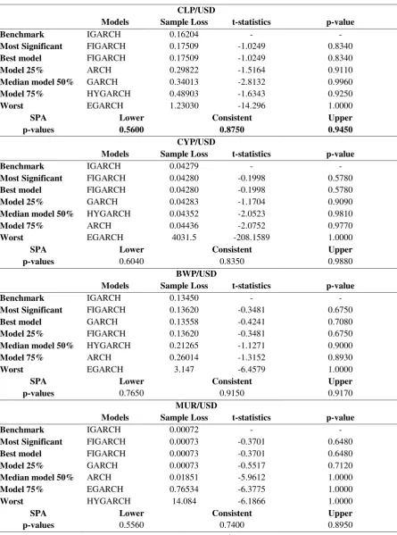
Table 11 presents the results obtained from the SPA test. The null hypothesis that the IGARCH model (the benchmark) is not inferior to each of the alternatives models cannot be rejected, according to the p-values of the last column of Table 11.13 In addition, two out of the three models (the IGARCH and the FIGARCH) that account for long memory dependencies in volatility persistence outperform the short memory models.

[Insert Table 11 here]

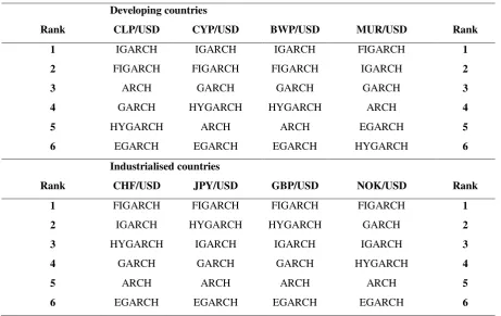
In Table 12 we provide a summary of the model rankings inferred from the SPA test results. In addition to the results for the developing countries we include results for our control group of industrialised countries.14 In the case of industrialised countries, the FIGARCH is consistently ranked first and which is line with the existing literature (see, e.g. Vilasuso, 2002).

[Insert Table 12 here]

In the case of the developing countries, IGARCH models tend to perform well both within sample and in out-of-sample forecasting. Models that capture long memory dependencies and persistence in volatility clearly outperform short memory models. The HYGARCH model estimates failed to satisfy the stationarity requirement, and rank poorly relative to IGARCH and FIGARCH in forecasting. Of the ARCH, GARCH and EGARCH models it there is strong evidence that accounting for asymmetries does not improve forecasting performance, in either the developing countries or industrialised countries under consideration. Our results for the developing countries make a new

13

We have also repeated the SPA test analysis with the FIGARCH as the benchmark model and tested whether forecasts from that specification are inferior to any of the other alternatives. These results strengthen the main thrust of our results and can be provided upon request.

14

18

contribution to an established literature, to the best of our knowledge this is the first paper focusing on the forecasting performance of developing countries’ exchange rate volatility with daily data. The fact that the IGARCH is found to be superior in out-of-sample forecast performance in developing countries (even though its difference in terms of performance with the FIGARCH is sometimes small) is important. The IGARCH model identifies infinite persistence of an exchange rate shock in developing countries.

3.4. Forecast Encompassing Tests

The results presented so far indicate that the FIGARCH and the IGARCH models are preferred in industrialised and developing countries, respectively, both on the basis of within-sample and out-of-sample performance. However, the difference is performance of these models is of interest, and that appears to be small in some cases. As a further check we carry out a forecast encompassing test to check whether the IGARCH (FIGARCH) model carries additional information over the base FIGARCH (IGARCH) model in industrialised (developing) countries. This forecast encompassing test was originally proposed by Chong and Hendry (1996) and is defined as

𝜎𝑡 =𝛼+𝛽1𝐹1,𝑡+𝛽2𝐹2,𝑡+𝜀𝑡, (12)

where 𝐹₁,𝑡 is the forecast attained from the first model and 𝐹2,𝑡 the forecast attained from the second

model. If 𝛽2 = 0, there is no incremental predictive information of the second model and thus, it is said that 𝐹₁,𝑡 encompasses 𝐹2,𝑡. However, if 𝛽2> 0 then the competing forecast, 𝐹2,𝑡, contains

information that 𝐹_1,𝑡 does not and therefore, it is said that 𝐹_1,𝑡 does not encompass 𝐹_2,𝑡. The null hypothesis that 𝛽2= 0, can be tested using a standard regression. The results of the forecast encompassing test are presented in Table 13.

19

In the case of the industrialised countries the (base) FIGARCH model encompasses the IGARCH model in all exchange return series apart from the CHF/USD series. This implies there is no additional information contained in the IGARCH model over the FIGARCH model, and adds supports to our previous results in Table 12. Turning to the results of the forecast encompassing test in developing countries the (base) IGARCH model encompasses the FIGARCH in all series except MUR/USD series. That is, apart from the MUR/USD series the FIGARCH does not contain any additional information over the IGARCH which again generally confirms our previous results in Table 12. In conclusion, the results of the forecast encompassing tests in developing and industrialised countries strengthens our previous finding that the FIGARCH and the IGARCH models are preferred in industrialised and developing countries, respectively.

4. Conclusion

The main objective of this research was to explore modelling and forecasting of exchange rate volatility in developing countries. The key question was whether the traditional univariate volatility models used widely and successfully in previous studies of industrialised countries perform equally well when applied to data for developing countries. The exchange rate series investigated in this study were the CLP/USD, CYP/USD, BWP/USD and MUR/USD in the case of developing countries and the CHF/USD, JPY/USD and GBP/USD and the NOK/USD in the case of our control group of industrialised countries. We reported estimation results for six competing volatility models.

20

In the case of developing countries’ exchange rate returns, the results of within-sample estimates, residual diagnostics and out-of-sample forecast evaluation indicate that the IGARCH model fits the data better than the FIGARCH, GARCH, HYGARCH, ARCH and EGARCH models and, in most cases, offers a superior performance in out-of-sample forecasting. The IGARCH model implies infinite persistence in the dispersion of exchange rate shocks. The FIGARCH model was found to rank second in order in terms of both in-sample estimation and out-of-sample forecasting performance.

In the case of developing countries these results address a gap in the existing literature on forecasting exchange rate volatility using daily data. To the best of our knowledge, there are no existing studies of developing countries’ data that focus on the forecasting performance of models that capture daily exchange rate volatility. Further work along these lines may be called for, to check that results are not specific to the particular data set and/or the specification in the volatility process. For instance, it would be of great interest to check whether our results for four developing countries can be generalised for a wider range of other developing countries, although at present our analysis focused on countries that have not been subject to a discrete change in their exchange rate regime during the sample. Extending the analysis to countries that have seen a regime change would be likely to require a multiple regime modelling approach that can potentially allow for structural changes in the volatility process over time.

21

References

Andersen, T. G. and Bollerslev T. 1998a. ‘Answering the Skeptics: Yes, Standard Volatility

Models Do Provide Accurate Forecasts’, International Economic Review, Vol.39 (4), pp.

885-905.

Andersen, T. G. and Bollerslev T. 1998b. ‘Deutsche Mark-Dollar Volatility: Intraday Activity

Patterns, Macroeconomic Announcements, and Longer Run Dependencies’, Journal of

Finance, Vol. 53 (1), pp. 219-265.

Andersen, T.G., Bollerslev T., Diebold F.X. and Labys P. 1999. ‘(Understanding, Optimizing,

Using and Forecasting) Realized Volatility and Correlation’, Working Paper Series, No

99-061, New York University, Leonard N. Stern School, Finance Department.

Andersen, T.G., Bollerslev T., Diebold F.X. and Labys P. 2001. ‘The Distribution of Realized

Exchange Rate Volatility’, Journal of the American Statistical Association, Vol. 96 (453), pp.

42-55.

Andersen, T.G., Bollerslev T., Diebold F.X. and Labys P. 2003. ‘Modeling and Forecasting

Realized Volatility’, Econometrica, Vol. 71 (2), pp. 579-625.

Baillie, R. T. and T. Bollerslev 1989. ‘Common Stochastic Trends in a System of Exchange

Rates’, Journal of Finance, Vol. 44 (1), pp 167-181.

Baillie, R. T., Bollerslev, T. and Mikkelsen, H. O. 1996. ‘Fractionally Integrated Generalized

Autoregressive Conditional Heteroskedasticity’, Journal of Econometrics, Vol. 74 (1), pp.

3-30.

Balaban, E. 2004. ‘Comparative Forecasting Performance of Symmetric and Asymmetric

Conditional Volatility Models of an Exchange Rate’, Economic Letters, Vol. 83 (1), pp.99-105.

Bollerslev, T. 1986 ‘Generalized Autoregressive Conditional Heteroskedasticity’, Journal of

22

Bollerslev, T. 1987. ‘A Conditionally Heteroskedastic Time Series Model for Speculative

Prices and Rates of Return’, The Review of Economics and Statistics, vol. 69 (3), pp. 542-47.

Bollerslev, T., Chou R. Y. and Kroner, K. F. 1992. ‘ARCH Modelling in Finance: A Review

of the Theory and Empirical Evidence’, Journal of Econometrics, Vol. 52 (1-2), pp. 55-59.

Bollerslev, T. and Mikkelsen, H. O. 1996. ‘Modeling and Pricing Long Memory in Stock

Market Volatility’, Journal of Econometrics, Vol. 73 (1), pp. 151-184.

Chong, Y. Y., and Hendry, D. F., 1986. ‘Econometric Evaluation of Linear Macro-Economic

Models’, Review of Economic Studies, Vol. 53 (4), pp. 671-90.

Cramer, J. S. 1986. ‘Econometric Applications of Maximum Likelihood Methods’,

Cambridge University Press, New York, NY.

Davidson, J. 2004. ‘Moment and Memory Properties of Linear Conditional Heteroskedasticity

Models, and a New Model’, Journal of Business and Economic Statistics, Vol. 22 (1), pp.

16-29.

Devereux, M. B. and Lane, P. R., 2003. ‘Understanding Bilateral Exchange Rate Volatility’,

Journal of International Economics, Vol. 60 (1), pp. 109-132.

Diebold F. X. and Inoue A. 2001. ‘Long Memory and Regime Switching’, Journal of

Econometrics, Vol. 105 (1), pp. 131–159.

Diebold, F. X. and Mariano, R. S. 1995. ‘Comparing Predictive Accuracy’, Journal of

Business and Economic Statistics, Vol. 13 (3), pp. 253-263.

Engle, R. F. 1982. ‘Autoregressive Conditional Heteroskedasticity with Estimates of the

Variance of United Kingdom Inflation’, Econometrica, Vol. 50 (4), pp. 987–1006.

Engle, R.F. and Bollerslev, T. 1986. ‘Modelling the Persistence of Conditional Variances’,

Econometric Reviews, Vol. 5 (1), pp. 1-50.

Goffe, W. L., Ferrier, G. D. and Rogers J. 1994. ‘Global Optimization of Statistical Functions

23

Hansen, P. R. 2005. ‘A Test for Superior Predictive Ability’, Journal of Business and

Economic Statistics, Vol 23, pp. 365-380.

Hansen, P. R. and Lunde, A. 2005. ‘A Forecast Comparison of Volatility Models: Does

Anything Beat a GARCH(1,1)?’, Journal of Applied Econometrics, Vol. 20 (7), pp. 873–889.

Hausmann R., Panizza U. and Rigobon R. 2006. ‘The Long-run Volatility Puzzle of the Real

Exchange Rate’, Journal of International Money and Finance, Vol. 25 (1), pp. 93-124.

Hsieh, D. 1989. ‘Modeling Heteroskedasticity in Daily Foreign-Exchange Rates’, Journal of

Business and Economic Statistics, Vol. 7 (3), pp. 307-317.

Kisinbay, T. 2010. ‘Predictive ability of asymmetric volatility models at medium-term

horizons’, Applied Economics, Vol. 42 (30), pp. 3813-3829.

Levy-Yeyati, E. and Sturzenegger, F. 2005. ‘Classifying Exchange Rate Regimes: Deeds Vs.

Words’, European Economic Review, Vol. 49 (6), pp. 1603-1635.

Martens M., Chang Y.-C. and S. J. Taylor, S. J. 2002. ‘A Comparison of Seasonal Adjustment

Methods When Forecasting Intraday Volatility’, Journal of Financial Research, Vol. 25 (2),

pages 283-299.

McCurdy, T., and Morgan, I. 1988. ‘Testing the Martingale Hypothesis in Deutsche Mark

Futures with Models Specifying the Form of Heteroskedasticity’, Journal of Applied

Econometrics, Vol. 3 (3), pp. 187-202.

Mincer J. and Zarnowitz V. 1969. ‘The Evaluation of Economic Forecasts’, in Mincer J (Eds),

‘Economic Forecasts and Expectations’, NBER, New York.

Nelson, D. B. 1991. ‘Conditional Heteroskedasticity in Asset Returns: A New Approach’,

Econmetrica, Vol. 59 (2), pp. 347-370.

Patton, A.J. 2011. ‘Volatility Forecast Comparison Using Imperfect Volatility Proxies’,

24

Pong, S., Shackleton, M. B., Taylor, S. J. and Xu, X. 2004. ‘Forecasting Currency Volatility:

A Comparison of Implied Volatilities and AR(FI)MA Models’, Journal of Banking and

Finance, Vol. 28 (10), pp. 2541-2563.

Poon, S.H. and Granger C. W. J. 2003. ‘Forecasting Volatility in Financial Markets: A

Review’, Journal of Economic Literature, Vol. 41 (2), pp. 478-539.

Tse, Y. K. 1998, ‘The Conditional Heteroscedasticity of the Yen-Dollar Exchange Rate’,

Journal of Applied Econometrics, Vol. 13 (1), pp. 49-55.

Vilasuso, J. 2002. ‘Forecasting Exchange Rate Volatility’, Economics Letters, Vol. 76, pp.

59-64.

25

CYP/USD BWP/USD CLP/USD MUR/USD Minimum -0.027509 -0.038329 -0.046232 -0.024876 Maximum 0.055115 0.073553 0.073225 0.029836 Mean 0.00012034 0.00044093 0.00024122 0.00023843 Standard Deviation 0.0053665 0.0052807 0.0045869 0.0036893

Skewness 0.281 [0.00]** 1.663 [0.00]** 1.805 [0.00]** 0.595 [0.00]** Excess Kurtosis 7.46 [0.00]** 28.66 [0.00]** 44.27 [0.00]** 10.16 [0.00]** JB Normality Test 4796 [0.00]** 71396 [0.00]** 1.69e+5[0.00]** 8968 [0.00]** ARCH 1-2 2.109 [0.12] 39.03 [0.00]** 48.86 [0.00]** 118.0 [0.00]** ARCH 1-5 1.957 [0.08] 19.75 [0.00]** 19.84 [0.00]** 50.09 [0.00]** ARCH 1-10 1.452 [0.15] 10.06 [0.00]** 10.63 [0.00]** 27.73 [0.00]** Q(5) 6.231 [0.28] 29.78 [0.00]** 31.84 [0.00]** 135.0 [0.00]** Q(10) 8.887 [0.54] 19.75 [0.00]** 37.83 [0.00]** 151.3 [0.00]** Q(20) 21.68 [0.36] 10.06 [0.00]** 59.69 [0.00]** 212.0 [0.00]** Q2(5) 11.00 [0.05] 133.0 [0.00]** 111.2 [0.00]** 340.9 [0.00]** Q2(10) 17.89 [0.06] 147.5 [0.00]** 121.1 [0.00]** 433.7 [0.00]** Q2(20) 36.66 [0.01]* 155.5 [0.00]** 132.3 [0.00]** 876.0 [0.00]**

26

Table 2. In-sample Estimation Results for CLP/USD - 08.11.1993-29.12.2000

ARCH GARCH EGARCH IGARCH FIGARCH HYGARCH C(M) 0.00003

(0.59) 0.00002 (0.32) 0.00002 (0.27) 0.00003 (0.59) 0.00004 (0.64) 0.00015 (2.04)*

C(V) 0.0904 (59.1)** 0.0061 (10.9)** 0.0997 (6.13)** 0.0097 (22.6)** 0.0342 (22.3)** -0.0178 (-14.7)**

AR(1) 0.1085 (4.27)** 0.0979 (5.52)** -68358.5 (-4494)** 0.1013 (4.17)** 0.1085 (4.05)** 0.1056 (4.80)**

α(1) 0.7376

(11.8)** 0.3611 (132)** -0.0779 (-43.9)** 0.1160 (37.6)** 0.3665 (4.12)** 0.4735 (397)**

α(4) 0.1195

(3.38)**

β(1) 0.8986

(600)**

0.9235 (797)**

0.8840 0.5723 (56.0)**

0.4042 (53.8)**

θ(1) 0.0197

(1.69)

θ(2) 0.5508

(239)**

Log(α) HYGARCH

1.9363 (79.6)**

Student-DF 2.4900 (47.3)** 2.2166 (166)** 2.2620 (977)** 2.5559 (56.2)** 2.5980 (49.3)**

Asymmetry 0.0644

(2.51)*

Tail 2.2052

(131)**

D 0.5368

(10.8)**

0.1565 (5.75)**

Log-Lik 7962.41 7990.79 7954.66 7973.47 7974.51 7998.31

AIC -8.8089 -8.8425 -8.8003 -8.8244 -8.8234 -8.8475

SBC -8.7845 -8.8242 -8.7759 -8.8092 -8.8021 -8.8201

HQC -8.7999 -8.8358 -8.7913 -8.8188 -8.8155 -8.8374

Shibata -8.8089 -8.8425 -8.8003 -8.8245 -8.8234 -8.8476

ARCH 1-5 0.4005 [0.85] 0.1421 [0.98] 0.1557 [0.98] 0.4426 [0.82] 0.1520 [1.00] 0.1360 [0.98]

ARCH 1-10 0.2379 [0.99] 0.1291 [1.00] 0.1156 [1.00] 0.2775 [0.99] 0.0918 [1.00] 0.0889 [1.00]

Q(10) 11.998 [0.21] 7.2272 [0.61] 8.4481 [0.49] 6.0108 [0.74] 8.7100 [0.46] 9.3735 [0.40]

Q(20) 29.913 [0.06] 16.092 [0.65] 23.653 [0.21] 18.854 [0.47] 24.111 [0.19] 22.092 [0.28]

Q2(10) 2.3451 [0.89] 1.3107 [1.00] 1.0986 [1.00] 2.8882 [0.94] 0.8954 [1.00] 0.8550 [1.00]

Q2(20) 8.2565 [0.94] 2.2582 [1.00] 4.1066 [1.00] 4.0039 [1.00] 3.0799 [1.00] 1.5020 [1.00]

27

Table 3. In-sample Estimation Results for CYP/USD - 08.11.1993-29.12.2000

ARCH GARCH EGARCH IGARCH FIGARCH HYGARCH C(M) 0.0002

(2.01)* 0.0002 (1.87) 0.0002 (1.55) 0.0002 (1.88) 0.0002 (1.90) 0.0001 (1.00)

C(V) 0.1329 (7.77)** 0.0007 (2.7)** -84471.7 (-58.7)** 0.0009 (3.73)** 0.0011 (1.38) -0.0022 (-2.12)*

AR(1) 0.0625 (2.79)** 0.0639 (3.2)** 0.0654 (3.01)** 0.0641 (2.98 )** 0.0658 (3.02)** 0.0662 (4.08)**

α(1) 0.0867

(2.04)** 0.0248 (10.2)** 0.4027 (1.24) 0.0346 (21.1)** 0.0812 (3.49)** 0.4593 (94.9)**

α(10) 0.0732

(1.98)*

β(1) 0.9665

(363)**

0.7077 (9.90)**

0.9654 0.9526 (47.7)**

0.8225 (94.3)**

θ(1) -0.0830

(-2.05)*

θ(2) 0.2121

(3.69)**

Log(α) HYGARCH

0.1208 (11.6)**

Student-DF 3.8612 (10.6)** 4.2163 (11.3)** 3.6272 (11.3)** 4.2755 (11.7)** 4.3565 (10.6)**

Asymmetry -0.0346

(-1.26)

Tail 4.0460

(10.2)**

D 0.9231

(26.1)**

0.3968 (61.4)**

Log-Lik 7156.49 7177.28 7132.32 7177.24 7178.02 7175.94

AIC -7.9097 -7.9416 -7.8896 -7.9427 -7.9413 -7.9368

SBC -7.8671 -7.9234 -7.8653 -7.9275 7.9200 -7.9094

HQC -7.8940 -7.9349 -7.8806 -7.9371 -7.9335 -7.9267

Shibata -7.9099 -7.9416 -7.8897 -7.9427 -7.9414 -7.9369

ARCH 1-5 0.54782 [0.74] 1.0138 [0.41] 0.6207 [0.68] 1.0045 [0.41] 0.4430 [0.82] 0.2330 [0.95]

ARCH 1-10 0.7518 [0.68] 0.6833 [0.74] 1.7733 [0.06] 0.6865 [0.74] 0.4160 [0.94] 0.4049 [0.95]

Q(10) 7.3725 [0.60] 7.8917 [0.55] 6.7672 [0.66] 7.8243 [0.55] 7.1080 [0.63] 7.0618 [0.63]

Q(20) 22.317 [0.27] 18.627 [0.48] 22.290 [0.27] 18.705 [0.48] 18.197 [0.51] 17.892 [0.53]

Q2(10) 7.4064 [1.00] 6.8040 [0.56] 17.9243 [0.02]* 6.8322 [0.55] 4.1529 [0.84] 4.0889 [0.85]

Q2(20) 20.008 [0.03]* 12.774 [0.80] 48.135 [0.00]** 12.774 [0.80] 10.853 [0.90] 11.886 [0.85]

28

Table 4. In-sample Estimation Results for BWP/USD - 08.11.1993-29.12.2000

ARCH GARCH EGARCH IGARCH FIGARCH HYGARCH C(M) 0.0002

(3.46)** 0.0002 (3.73)** 0.0002 (4.68)** 0.0002 (3.85)** 0.0002 (3.78)** 0.0003 (3.94)**

C(V) 0.0916 (62.7)** 0.0234 (30.3)** -62956.87 (-462)** 0.0229 (38.2)** 0.0194 (24.9)** 0.0095 (2.11)*

AR(1) -0.0400 (-1.68) -0.0353 (-1.42) -0.0317 (-11.6)** -0.0393 (-1.94) -0.0414 (-1.84) -0.0476 (-2.35)*

α(1) 0.8733

(6.86)** 0.2811 (16.3)** -0.0214 (-6.82)** 0.3013 (87.3)** 0.4078 (55.7)** 0.5681 (56.6)**

α(4) 0.4262

(4.08)**

β(1) 0.7023

(193)**

0.8705 (586)**

0.3864 0.6972 (460)**

0.7060 (30.6)**

β(2) 0.3124

(6.03)**

θ(1) 0.1844

(12.0)**

θ(2) 0.7567

(190)**

Log(α) HYGARCH

0.6014 (65.1)**

Student-DF 2.4349 (52.2)** 2.7956 (37.4)** 2.4273 (696)** 2.7439 (41.8)** 2.7719 (40.4)**

Asymmetry 0.0380

(1.62)

Tail 2.4236

(71.2)**

D 0.6557

(304)**

0.5236 (23.8)**

Log-Lik 7659.89 7662.11 7648.69 7666.08 7671.73 7684.4

AIC -8.4739 -8.4785 -8.4615 -8.4829 -8.4881 -8.4999

SBC -8.4495 -8.4603 -8.4371 -8.4647 -8.4668 -8.4725

HQC -8.4649 -8.4718 -8.4525 -8.4762 -8.4802 -8.4898

Shibata -8.4739 -8.4785 -8.4615 -8.4829 -8.4881 -8.4999

ARCH 1-5 0.7642 [0.58] 1.4715 [0.20] 0.5694 [0.72] 1.3982 [0.22] 1.6457 [0.15] 0.4973 [0.78]

ARCH 1-10 0.8913 [0.54] 0.8934 [0.54] 0.5297 [0.87] 0.8321 [0.60] 0.9307 [0.50] 0.4153 [0.94]

Q(10) 18.881 [0.03]* 18.413 [0.03]* 17.705 [0.04]* 10.6442 [0.29] 18.605 [0.03]* 17.949 [0.04]*

Q(20) 34.649 [0.02]* 30.595 [0.04]* 30.648 [0.04]* 22.326 [0.07] 30.392 [0.05]* 31.782 [0.03]*

Q2(10) 8.7647 [0.19] 9.2648 [0.32] 5.3619 [0.72] 8.6153 [0.28] 10.162 [0.25] 4.3338 [0.83]

Q2(20) 27.185 [0.04]* 34.999 [0.01]** 24.997 [0.12] 25.675 [0.08] 23.870 [0.15] 14.457 [0.70]

29

Table 5. In-sample Estimation Results for MUR/USD - 08.11.1993-29.12.2000

ARCH GARCH EGARCH IGARCH FIGARCH HYGARCH C(M) 0.0001

(4.57)** 0.0001 (4.70)** 0.0001 (2.98)** 0.0001 (4.64)** 0.0001 (4.67)** 0.0001 (2.84)**

C(V) 0.0736 (40.7)** 0.0271 (42.7)** -1585.257 (-512)** 0.0144 (57.3)** 0.0378 (52.4)** -0.6202 (-1542)**

AR(1) -0.0881 (-10.5)** -0.0865 (-3.74)** -0.0664 (-3.28)** -0.0742 (-3.58)** -0.0843 (-3.28)** -0.0980 (-21.3)**

α(1) 1.0000

(11.9)** 0.2534 (9.26)** 0.5492 (1.47)** 0.1525 (112)** 0.2556 (2.58)** 0.0195 (14.4)**

α(10) 1.0000

(2.12)*

β(1) 0.7245

(134)**

0.9800 (227)**

0.4099 0.5943 (77.4)**

0.4017 (299)**

β(2) 0.4375

(7.27)**

θ(1) 0.1332

(0.75)

θ(2) 1.2006

(4.54)**

Log(α) HYGARCH

4.8484 (4410)**

Student-DF 2.0751 (220)** 2.2976 (77.2)** 2.0110 (728 )** 2.2776 (93.9)** 2.2856 (91.1)**

Asymmetry 0.0138

(1.05)

Tail 2.0037

(8517)**

D 0.5928

(6.37)**

0.3684 (620)**

Log-Lik 8316.77 8216.96 8338.1 8226.46 8226.49 8388.33

AIC -9.1945 -9.0930 -9.2249 -9.1035 -9.1024 -9.2794

SBC -9.1520 -9.0747 -9.2006 -9.0852 -9.0811 -9.2520

HQC -9.1789 -9.0862 -9.2159 -9.0968 -9.0946 -9.2693

Shibata -9.1948 -9.0930 -9.2249 -9.1035 -9.1025 -9.2795

ARCH 1-5 0.2532 [0.94] 0.4698 [0.80] 0.0898 [0.99] 1.7481 [0.12] 0.8378 [0.52] 0.4683 [0.80]

ARCH 1-10 0.4104 [0.94] 1.4780 [0.14] 0.0968 [1.00] 1.7712 [0.06] 1.7319 [0.07] 0.6913 [0.73] Q(10) 10.290

[0.33] 10.853 [0.29] 12.378 [0.19] 13.891 [0.13] 11.626 [0.23] 10.300 [0.33] Q(20) 30.877

[0.04] 36.921 [0.01]** 32.948 [0.02]* 25.392 [0.12] 36.182 [0.01]* 27.024 [0.10] Q2(10) 4.4342

[1.00] 15.020 [0.06] 0.9605 [1.00] 8.653 [0.98] 18.033 [0.02]* 6.8431 [0.55] Q2(20) 56.968

[0.00]** 77.137 [0.00]** 26.885 [0.08] 16.430 [0.29] 71.756 [0.00]** 23.864 [0.16]

30

Table 6. Mincer-Zarnowitz regression of

y

α β R2 Rank

ARCH 0.0001 (3.495)** [1.5782e-005]

0.1552 (1.141) [0.1360]

0.0246 2

GARCH 0.00005 (3.776)** [1.2580e-005]

0.1003 (1.401) [0.0716]

0.0115 6

EGARCH -0.0002 (-1.427) [0.00010417]

0.0645 (1.754) [0.0367]

0.0273 1

IGARCH 0.00005 (3.774)** [1.2580e-005]

0.3474 (1.354) [0.257]

0.0122 5

FIGARCH 0.00005 (2.914)** [1.8274e-005]

0.2820 (1.181) [0.2387]

0.0148 4

HYGARCH 0.00005 (2.697)** [1.8699e-005]

0.0866 (1.194) [0.0725]

0.0161 3

Notes: Numbers in brackets and parenthesis are White (1980) Heteroskedastic Consistent S.E. and t-values respectively. * Significant at 5%; ** significant at 1%.

Table 7. Mincer-Zarnowitz regression of

y

α β R2 Rank

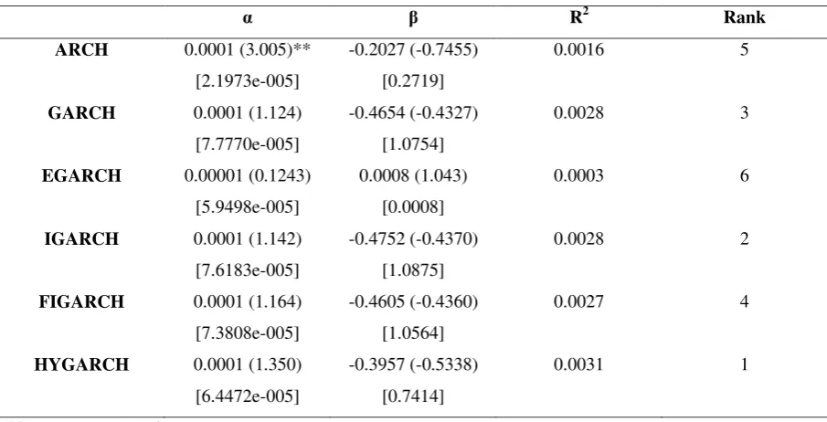
ARCH 0.0001 (3.005)** [2.1973e-005]

-0.2027 (-0.7455) [0.2719]

0.0016 5

GARCH 0.0001 (1.124) [7.7770e-005]

-0.4654 (-0.4327) [1.0754]

0.0028 3

EGARCH 0.00001 (0.1243) [5.9498e-005]

0.0008 (1.043) [0.0008]

0.0003 6

IGARCH 0.0001 (1.142) [7.6183e-005]

-0.4752 (-0.4370) [1.0875]

0.0028 2

FIGARCH 0.0001 (1.164) [7.3808e-005]

-0.4605 (-0.4360) [1.0564]

0.0027 4

HYGARCH 0.0001 (1.350) [6.4472e-005]

-0.3957 (-0.5338) [0.7414]

0.0031 1

31

Table 8. Mincer-Zarnowitz regression of

y

α Β R2 Rank

ARCH 0.00004 (1.888) [2.2252e-005]

-0.0132 (-0.9897) [0.0133]

0.00021 6

GARCH 0.00004 (1.875) [2.2828e-005]

-0.0465 (-1.095) [0.0425]

0.00033 3

EGARCH 0.0001 (1.179) [6.5229e-005]

-0.0222 (-0.8012) [0.0277]

0.0022 1

IGARCH 0.00004 (1.869) [2.3142e-005]

-0.0552 (-1.099) [0.0502]

0.0004 2

FIGARCH 0.00004 (1.873) [2.2795e-005]

-0.0433 (-0.9833) [0.0441]

0.00029 5

HYGARCH 0.00004 (1.869) [2.2828e-005]

-0.0197 (-0.9484) [0.0207]

0.00031 4

Notes: see Table 6.

Table 9. Mincer-Zarnowitz regression of

y

, for MUR/USD, on a constant and 1-step

out-of-sample forecasts (k=253)

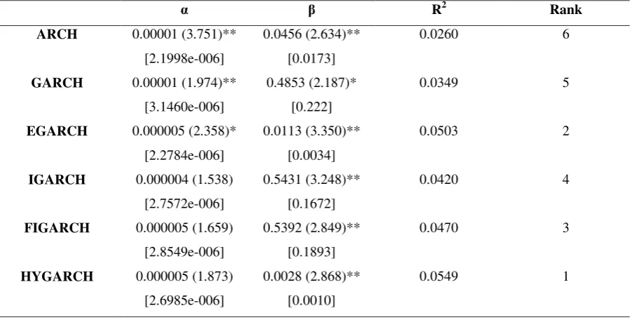
α β R2 Rank

ARCH 0.00001 (3.751)** [2.1998e-006]

0.0456 (2.634)** [0.0173]

0.0260 6

GARCH 0.00001 (1.974)** [3.1460e-006]

0.4853 (2.187)* [0.222]

0.0349 5

EGARCH 0.000005 (2.358)* [2.2784e-006]

0.0113 (3.350)** [0.0034]

0.0503 2

IGARCH 0.000004 (1.538) [2.7572e-006]

0.5431 (3.248)** [0.1672]

0.0420 4

FIGARCH 0.000005 (1.659) [2.8549e-006]

0.5392 (2.849)** [0.1893]

0.0470 3

HYGARCH 0.000005 (1.873) [2.6985e-006]

0.0028 (2.868)** [0.0010]

0.0549 1

32

Table 10. 1-step Out-of-Sample Forecast Evaluation Developing Countries (k=253)

MSFE

CLP/USD Rank CYP/USD Rank BWP/USD Rank MUR/USD Rank

ARCH 0.2500 3 0.0452 5 0.2553 5 0.0188 4

GARCH 0.3100 4 0.0434 3 0.1317 2 0.0008 3

EGARCH 12.2100 6 4031 6 3138 6 0.7656 5

IGARCH 0.1500 1 0.0434 1 0.1307 1 0.0008 2

FIGARCH 0.1600 2 0.0434 2 0.1323 3 0.0008 1

HYGARCH 0.4300 5 0.0440 4 0.2082 4 14.0900 6

33

Table 11. SPA test results evaluated by MSFE – Developing Countries

CLP/USD

Models Sample Loss t-statistics p-value

Benchmark IGARCH 0.16204 - -

Most Significant FIGARCH 0.17509 -1.0249 0.8340

Best model FIGARCH 0.17509 -1.0249 0.8340

Model 25% ARCH 0.29822 -1.5164 0.9110

Median model 50% GARCH 0.34013 -2.8132 0.9960

Model 75% HYGARCH 0.48903 -1.6343 0.9250

Worst EGARCH 1.23030 -14.296 1.0000

SPA Lower Consistent Upper

p-values 0.5600 0.8750 0.9450

CYP/USD

Models Sample Loss t-statistics p-value

Benchmark IGARCH 0.04279 - -

Most Significant FIGARCH 0.04280 -0.1998 0.5780

Best model FIGARCH 0.04280 -0.1998 0.5780

Model 25% GARCH 0.04283 -1.1704 0.9090

Median model 50% HYGARCH 0.04352 -2.0523 0.9810

Model 75% ARCH 0.04436 -2.0752 0.9770

Worst EGARCH 4031.5 -208.1589 1.0000

SPA Lower Consistent Upper

p-values 0.6040 0.8350 0.9880

BWP/USD

Models Sample Loss t-statistics p-value

Benchmark IGARCH 0.13450 - -

Most Significant FIGARCH 0.13620 -0.3481 0.6750

Best model GARCH 0.13558 -0.4241 0.7080

Model 25% FIGARCH 0.13620 -0.3481 0.6750

Median model 50% HYGARCH 0.21265 -1.1271 0.9000

Model 75% ARCH 0.26014 -1.3152 0.8930

Worst EGARCH 3.147 -6.4579 1.0000

SPA Lower Consistent Upper

p-values 0.7650 0.9150 0.9170

MUR/USD

Models Sample Loss t-statistics p-value

Benchmark IGARCH 0.00072 - -

Most Significant FIGARCH 0.00073 -0.3701 0.6480

Best model FIGARCH 0.00073 -0.3701 0.6480

Model 25% GARCH 0.00073 -0.5517 0.7120

Median model 50% ARCH 0.01851 -5.9612 1.0000

Model 75% EGARCH 0.76534 -6.3775 1.0000

Worst HYGARCH 14.084 -6.1866 1.0000

SPA Lower Consistent Upper

p-values 0.5560 0.7400 0.8950

34

Developing countries

Rank CLP/USD CYP/USD BWP/USD MUR/USD Rank

1 IGARCH IGARCH IGARCH FIGARCH 1

2 FIGARCH FIGARCH FIGARCH IGARCH 2

3 ARCH GARCH GARCH GARCH 3

4 GARCH HYGARCH HYGARCH ARCH 4

5 HYGARCH ARCH ARCH EGARCH 5

6 EGARCH EGARCH EGARCH HYGARCH 6

Industrialised countries

Rank CHF/USD JPY/USD GBP/USD NOK/USD Rank

1 FIGARCH FIGARCH FIGARCH FIGARCH 1

2 IGARCH HYGARCH HYGARCH GARCH 2

3 HYGARCH IGARCH IGARCH IGARCH 3

4 GARCH GARCH GARCH HYGARCH 4

5 ARCH ARCH ARCH ARCH 5

6 EGARCH EGARCH EGARCH EGARCH 6

Table 13. Forecast encompassing test: FIGARCH and IGARCH

Industrialised countries Developing countries

FIGARCH IGARCH IGARCH FIGARCH

CHF/USD -0.30 (-0.34) 1.29 (2.06)* CLP/USD 0.64 (2.01)* 0.31 (0.98)

JPY/USD 1.12 (3.12)** 0.09 (0.54) CYP/USD 0.57 (1.99)* 0.41 (1.45)

GBP/USD 0.88 (2.26)* 0.10 (0.65) BWP/USD 0.89 (3.34)** 0.08 (0.73)

NOK/USD 0.67 (1.99)* 0.25 (1.43) MUR/USD 0.16 (0.32) 0.84 (2.49)*