On the Homotopy Analysis Method and Optimal Value of
the Convergence Control Parameter: Solution of
Euler-Lagrange Equation
Jafar Saberi-Nadjafi, Reza Buzhabadi, Hassan Saberi Nik*
Department of Applied Mathematics, School of Mathematical Sciences, Ferdowsi University of Mashhad, Mashhad, Iran Email: *saberi [email protected]
Received May 19, 2012; revised June 20, 2012; accepted June 27, 2012
ABSTRACT
This paper presents, an efficient approach for solving Euler-Lagrange Equation which arises from calculus of variations. Homotopy analysis method to find an approximate solution of variational problems is proposed. An optimal value of the convergence control parameter is given through the square residual error. By minimizing the square residual error, the optimal convergence-control parameters can be obtained. It is showed that the homotopy analysis method was valid and feasible to the study of variational problems.
Keywords: Homotopy Analysis Method; Calculus of Variations; Variational Problems; Euler-Lagrange Equation; Square Residual Error
1. Introduction
There has been a considerable renewal of interest in the classical problems of the calculus of variations both from the point of view of mathematics and of applications in physics, engineering, and applied mathematics. The di- rect method of Ritz and Galerkin in solving variational problems has been of considerable concern and is well covered in many textbooks [1-3]. Chen and Hsiao [4] introduced the Walsh series method to variational prob- lems. Due to the nature of the Walsh functions, the solu- tion obtained were piecewise constant. Razzaghi [5] ap- plied the Fourier series, to derive a continuous solution for the second example in [4] which is an application to the heat conduction problem. Very recently, Dehghan and Tatari applied the Adomian decomposition method and variational iteration method to solve variational problems in [6,7], respectively and Abdulaziz, Hashim and Chowdhury applied the homotopy perturbation method to solve variational problems in [8].
One of the semi-exact methods for solving nonlinear Equation which does not need small/large parameters is HAM, first proposed by Liao in 1992 [9-13]. Since Liao [10] for the homotopy analysis method was published in 2003, more and more researchers have been successfully applying this method to various nonlinear problems in science and engineering, such as the viscous flows of non-Newtonian fluids [14], the KdV-type equations [15],
finance problems [16], nonlinear optimal control pro- blems [17] and so on.
The HAM contains a certain auxiliary parameter which provides us with a simple way to adjust and con- trol the convergence region and rate of convergence of the series solution. Moreover, by means of the so-called -curve, it is easy to determine the valid regions of to gain a convergent series solution. Thus, through HAM, explicit analytic solutions of nonlinear problems are pos- sible. In this paper, we will adopt the homotopy analysis method (HAM), for solving the Euler-Lagrange equation, which arises from problems in calculus of variations.
h
h h
2. Basic Idea of HAM
To describe the basic ideas of the HAM, we consider the following differential Equation
= 0,N u (1)
where N is a nonlinear operator, denotes indepen- dent variable, u
is an unknown function, respect-tively. For simplicity, we ignore all boundary or initial conditions, which can be treated in the similar way. By means of generalizing the traditional homotopy method, Liao [9] constructs the so-called zero-order deformation Equation
1q L
;q u0
=qhH
N
;q
, (2)a non-zero auxiliary parameter, is an auxil- iary function, is an auxiliary linear operator,
0
H
L u0
is an initial guess of u
, is a unknownfunction, respectively. It is important, that one has great freedom to choose auxiliary things in HAM. Obviously, when and , it holds
;q = 0
q q= 1
;0 =u0
, ;1 =u
,
q
(3) respectively. Thus, as increases from 0 to 1, the solution
;q
varies from the initial guess u0
tothe solution u
. Expanding u0
in Taylor serieswith respect to q, we have
0;q =u
m
m,m
u q
=1
(4)
where
=0; =
m
m
m q
=1
=
m
1
. !
q
,
m
q
u
u (5)
If the auxiliary linear operator, the initial guess, the auxiliary parameter and the auxiliary function are so properly chosen, the series (4) converges at , then we have
h
= 1
q
0 m
u u
(6)which must be one of solutions of original nonlinear equation, as proved by Liao [10]. As h=1 and
, Equation (2) becomes
H = 1
1q L
;q
u0
;q
0 1= u ,u
q N
, ,
n un
= 0,
(7)
which is used mostly in the homotopy perturbation method [18], where as the solution obtained directly, without using Taylor series. According to the definition (5), the governing equation can be deduced from the zero-order deformation Equation (2). Define the vector
.
m
!
1 =hH
u
Differentiating Equation (2) times with respect to the embedding parameter and then setting and finally dividing them by , we have the so-called
th-order deformation Equation
q
m
= 0
q
m m
m mu Rm um1 ,
L u (8)
where
11 1
;
m
N q
m q
1, > 1.
m u
=0
1 =
1 !
m
q
. (9)
m m
R u
and
0, =
1,
m
m m
(10)
It should be emphasized that
for isgoverned by the linear Equation (8) under the linear boundary conditions that come from original problem, which can be easily solved by symbolic computation software such as Matlab. For the convergence of the above method we refer the reader to Liao’s work. If Equation (1) admits unique solution, then this method will produce the unique solution.
1
m
Remark 1. In 2007, Yabushita et al. [19] applied the HAM to solve two coupled nonlinear ODEs, and sug- gested the so-called optimization method to find out two optimal convergence-control parameters by means of the minimum of the square residual error integrated in the whole region having physical meanings. Their approach is based on the square residual error
2=0
= M k d
k
h N u ,
(11)of a nonlinear Equation , where
=0
k
= 0 N u
M k
u
gives the M th-order HAM approximation.Obviously,
h 0 (as ) corresponds to a convergent series solution. For given orderM
M of
approximation, the optimal value of is given by a nonlinear algebraic equation
h
d
= 0, d
h h
We use exact square residual error (11) integrated in the whole region of interest , at the order of approxi-mation M.
3. Statement of the Problem
Let us consider the simplest form of the variational pro- blems
1
0= x , ,
x
y x F x y x y x x
d , (12)where is the functional whose extremum must be found. In order to find the extreme value of , the boundary conditions of the admissible curves are given by
0 = ,
1 = ,y x b y x a (13) The necessary condition for the solution to problem (12) is to satisfy the Euler-Lagrange equation:
d = 0, d
y y
F F
x
(14)
with the boundary conditions given in (13).
d ,nonlinear parts of the equation. unique. Also this unique extremal will be the solution of
the given variational problem. From Equation (20), we define the nonlinear operator The form of a variational problem involving two
de-rivative can be considered as
2
3 2
;
; = x q ; 8 x,
N x q x q e
x
(21)
1
0= x , , ,
x
y x F x y x y x y x x
(15) According to the initial condition denoted by (19), it is natural to choosewhere is the functional that its extremum must be found. To find the extreme value of , the boundary conditions of the admissible curves are known in the fol-lowing form
30 = .
x
y x e
We choose the linear operator
2
2;
; = x q ,
L x q
x
(22)
0 1 1 2
0 3 1
= , = , = , =
y x y x
y x y x 4.
(16)
with the property L c
1c x2
= 0 , where arecoefficient. 1 2
, c c where i, = 1, 2,3, 4i are known.
The necessary condition for the solution of the
prob-lem (15) is to satisfy the Euler-Lagrange Equation mAs mentioned in Section 2, we get the so-called th-order deformation equation:
2 2
d d
= 0,
d d
F F F
y x y x y
(17) L y m
x mym1
x =hH x R
m ym1
,where with boundary conditions given in (16).
2 1
31 = 2 1 1 8 .
x m
m m m m
y
R y e
x
y The Euler-Lagrange equations (14), (17) are in general
a nonlinear differential equation, which does not always
have an analytic solution. Now, the terms of the HAM solution can be given by
4. Numerical Results
30 = x, n = 0, = 1, 2,3,
y e y n
Hence, the solution to (20) is
= 3xy x e which is the exact solution.
To demonstrate the effectiveness of the HAM algorithm discussed above, several examples of variational
prob-lems will be studied in this section. Example 4.2. We consider the following brachisto-chrone problem:
Example 4.1. We consider the following variational problem:
2 2 1 0
1
min = d ,
1
y x
x y x
(23)
21 3
0
min = 4 x d ,
y x y x e x
e
,
(18)
subject to the boundary conditions subject to the boundary conditions
0 = 1, 1 = .
3y y (19) y
0 = 0, 1 = 0.5.y
(24) The corresponding Euler-Lagrange Equation is givenby The corresponding Euler-Lagrange Equation is given by
2
1 =
2 1
y
y ,
y
(25)
3 8 x= 0
y y e (20) subject to the boundary conditions (19).
To solve Equation (20) by means of HAM, we
con-sider the following process after separating the linear and with boundary conditions (24). The exact solution to the brachistochrone problem (23) in implicit form is
22
, = 0.381510869 0.618489131
0.1907554345
0.8092445655arctan 0.5938731505 = 0.
0.381510869 0.618489131
F x y y y
y
x
y y
follows: Following Zhang and He [20], we can expand the non-
linear term
11y in (25) using the Taylor series as
2
1
Hence, we can rewrite the Euler-Lagrange Equation (25) as follows:
2 2 2 2 2
1 = 1
2
y y y y yy y y , (26)
To solve Equation (26) by means of HAM, we define the nonlinear operator
2
2 2
2
2 2
2
; 1
; = ; ;
2
1 1
; ;
2 2
1 1 1
; ; .
2 2 2
x q
N x q x q x q
x
;
x q x q x q
x q x q
From the initial conditions (24), the initial guess is
20
1 = .
2
y x x
As mentioned in Section 2, we get the so-called th-order deformation equation with
m
2 1
1
1 2 1
=0 =0 =0
1
1 =0 =0
1
1 =0
1
1 1
=0
1
= ,
2 1
2
1 ,
2
1 1 1 1 .
2 2 2
j
m k
j i
m i
m m m k k j
k j i
m k
j k j
m k
k j
m
k m k
k
m
k m k m m
k
y y
R y y y
x x
x
y y
y
x x
y y
x x
y y y
y
Now, the terms of the HAM solution can be given by
2 4 6 8
1
2 4 6 8
2
2 2 3
5 6 7
10
5167 3 1 1 1
= ,
6720 4 48 240 448
5167 3 1 1 1
=
6720 4 48 240 448
320585329 3 5167 11
403603200 4 80640 96
5167 77 5167 389
268800 2880 376320 26880
271 29
403200
y h x x x x x
y h x x x x x
h x x x 4
8
x
x x x
x
x
12 14
4 3
5
221760 163072
1 1 1
.
448 448 448
x x
x x x
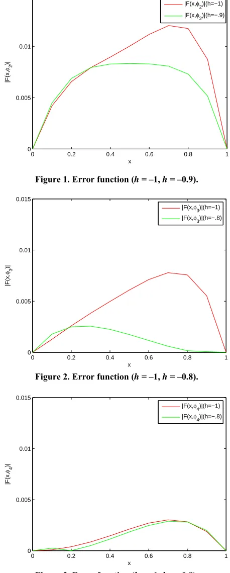
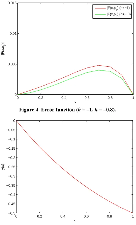
In Figures 1-4, we plot the comparison of error func-
tion F x
,m
for with .Figure 5 shows the 4-term HAM approximate solution = 2,3, 4,5
m h= 1, 0.9, 0.8
4 x
of (26). When , it is easily seen that the solutions above are exactly the solutions in [8]. Therefore, the HPM solution is indeed a special case of the HAM solution when .
= 1
h
1
= h
By HAM, it is easy to discover the valid region of h, which corresponds to the line segments nearly parallel to the horizontal axis. To find a proper value of the - curve of given by the 8th-order HAM appro-
h h
(0.1)
y
0 0.2 0.4 0.6 0.8 1
0 0.005 0.01 0.015
x
|F(
x
,
φ2
)|
|F(x,φ2)|(h=−1)
[image:4.595.307.536.155.725.2]|F(x,φ2)|(h=−.9)
Figure 1. Error function (h = –1, h = –0.9).
0 0.2 0.4 0.6 0.8 1
0 0.005 0.01 0.015
x
|F(
x
,
φ3
)|
|F(x,φ3)|(h=−1) |F(x,φ3)|(h=−.8)
Figure 2. Error function (h = –1, h = –0.8).
0 0.2 0.4 0.6 0.8 1
0 0.005 0.01 0.015
x
|F(
x
,
φ4
)|
|F(x,φ4)|(h=−1)
|F(x,φ4)|(h=−.8)
0 0.2 0.4 0.6 0.8 1 0
0.005 0.01 0.015
x
|F(
x
,
φ5
)|
[image:5.595.63.538.73.789.2]|F(x,φ5)|(h=−1) |F(x,φ5)|(h=−.8)
Figure 4. Error function (h = –1, h = –0.8).
0 0.2 0.4 0.6 0.8 1
−0.5 −0.45 −0.4 −0.35 −0.3 −0.25 −0.2 −0.15 −0.1 −0.05 0
x
y(x)
Figure 5. The 4th-order HAM results.
ximation is drawn in Figure 6, which clearly indicates that the valid region of h is about 1.4 h 0.2.
As mentioned in Section 2, the optimal value of is determined by the minimum of , corresponding to the
h
5
nonlinear algebraic Equation d 5 = 0
dh
. Our calculations
showed that, 5 has its minimum value at –0.9.
Example 4.3. We consider the following variational problem:
π2 2
2 0
min ,
= 2
y x z x
y x z x y x z x x
d ,(27)
subject to the boundary conditions
0 = 0, π = 1, 0 = 0,
π = 1.2 2
y y z z
(28)
The corresponding system of Eulers differential equa-tions is given by
= 0, = 0,
yz zy (29)
−2.5 −2 −1.5 −1 −0.5 0 0.5 1 1.5
−5 0 5 10
h
[image:5.595.59.287.84.459.2]y(.1)
Figure 6. The h-curve of y(0.1) 8th-order HAM.
with boundary conditions (28). The exact solution to the variational problem (27) is as follows [6]:
= sin
, = sin
.y x x z x x
To solve the Equations (29) by means of homotopy analysis method, we choose the initial guess
0 0= sin cos ,
= sin cos .
y x A x B x
z x C x D x
(30)
We now define a nonlinear operators as:
2 1
1 1 2 2 2
2 2
2 1 2 2 1
;
; , ; = ; ,
;
; , ; = ; .
x q
N x q x q x q
x
x q
N x q x q x q
x
As mentioned in Section 2, we get the so-called th- order deformation Equation with
m
21
1, 1 2 1
2 1
2, 1 2 1
= ,
= ,
m
m m m
m
m m m
y
R z
x z
R y
x
y
z
and initial conditions:
0 = 0; 0 = 0, 0 = 0; 0 = 0.
m m x
m m x
y y
z z
We start with an initial approximation we can obtain directly the other components as: 0 0
,
y z
1
2
= s
cos sin cos ,
= 1 sin
cos sin cos ,
y h B D Ax Cx A x
B x C x D x
y h h B D Ax Cx A
B x C x D x
in
[image:5.595.311.535.85.263.2]
1
2
= s
cos sin cos ,
= 1 sin
cos sin cos ,
z h B D Ax Cx A x
B x C x D x
z h h B D Ax Cx A
B x C x D x
in
x
Imposing the boundary conditions on and , we
obtain . Hence with
1
y z1
=
h
= 1, = 0,
A B C= 1, = 0 D 1,
the exact solution of the problem will be obtained. In
Figures 7 and 8, we compare the exact solution
,y x z x
0 t 1
with the 2-term HAM approximate solution, for . Figures 9 and 10 shown the -curve of h
π , π
4 4
y z
given by the 8th-order HAM approxi-
mation.
As mentioned in Section 2, the optimal value of is determined by the minimum of , corresponding to the
h
2
0 0.5 1 1.5
0 0.1 0.2 0.3 0.4 0.5 0.6 0.7 0.8 0.9 1
x
y(
x)
[image:6.595.311.535.85.519.2]HAM Exact
Figure 7. Comparison between the HAM solution of y(x) and the exact solution.
0 0.5 1 1.5
−1 −0.9 −0.8 −0.7 −0.6 −0.5 −0.4 −0.3 −0.2 −0.1 0
x
z(
x)
HAM Exact
Figure 8. Comparison between the HAM solution of z(x) and the exact solution.
−3 −2.5 −2 −1.5 −1 −0.5 0 0.5 1
0 0.5 1 1.5 2 2.5 3
h
y(
π
/4)
Figure 9. The h-curve of
π , = 10
4
y n .
−3 −2.5 −2 −1.5 −1 −0.5 0 0.5 1
−3 −2.5 −2 −1.5 −1 −0.5 0 0.5
h
z(
π
[image:6.595.62.286.325.497.2]/4)
Figure 10. The h-curve of
π , = 10
4
z n .
nonlinear algebraic Equation d 2 = 0
dh
. Our calculations
showed that, 2 has its minimum value at 1.
Example 4.4. In this example we consider the varia- tional problem
1
2
2
0min =y x
y x y x d ,x (31)subject to the boundary conditions
0 = 0, 0 = 1,
1 = sinh 1 , 1 = cosh 1 ,
y y
y y
(32)
which has the the exact solution y x
= sinh
x .The Euler-Lagrange Equation of this problem can be written in the following form
(4) = 0.
y x y x (33)
[image:6.595.61.284.536.707.2]this problem,we consider the transformation
1
2
2 3
3 4
d d d
= , = , = , = ,
d d d
y y y
y x y x y x y x y x
x x x
we rewrite the above fourth-order boundary value prob-lem as a system of differential equations
1 2 d = d y y xx , (34)
2 3 d = d y y xx , (35)
3 4 d = d y y xx , (36)
4 3 d = d y y xx , (37)
To solve Equations (34)-(37) by means of the HAM, we choose the initial approximations
1,0 = 0, 2,0 = 1, 3,0 = , 4,0 = .
y x y x y x A y x B (38)
Furthermore, we define a system of nonlinear opera- tors as
1 1 2 2 2 3 3 3 4 4 4 3 ; ; = ; , ; ; = ; ; ; = ; ; ; = ; ) i i i i x qN x q x q
x x q
N x q x q
x x q
N x q x q
x x q
N x q x q
x , , .
As mentioned in Section 2, we get the so-called th- order deformation Equation with
m
1, 11, 1, 1 2, 1
2, 1
2, 2, 1 3, 1
3, 1
3, 3, 1 4, 1
4, 1
4, 4, 1 3, 1
= ,
= ,
= ,
= .
m
m m m
m
m m m
m
m m m
m
m m m
y R y x y R y x y R y x y R y x y y y y
We start with an initial approximation, we can obtain directly the other components as:
1,1 = ,
y x hx
1,2
1
= 2 2 2
y x hx hhAx ,
1,32 2 2 2
1
= 6 12 6 6 6
3
y x
hx h hAx h x B h xA h
2 2 2
1,4
2 3 3 3 2 3 3
1
= 24 72 36 12 72 24
72 12 36 24 ,
y x hx h hAx h x B h xA
h h Ax h Bx xh A h
2,1 = ,
y x hAx
2,2
1
= 2 2
2 ,
y x hx A hA hxB
2,3
2 2 2 2
( ) 1
= 6 12 6 6 6
6
y x
hx A hA hxB h Ax h xB h A
,
3,1 = ,
y x hBx
3,2
1
= 2 2 2
y x hx B hBhAx
,
4,1 = ,
y x hAx
4,2
1
= 2 2
2 ,
y x hx A hA hxB
4,3
2 2 2 2
1
= 6 12 6 6 6
6
y x
hx A hA hxB h Ax h xB h A
,
when h= 1 , it is easily seen that the solutions above
are exactly the solutions in [6],
7 1,
2 3 4 5=1 n 2! 3! 4! 5!
= .
n
Ax Bx Ax Bx
y x
y x x on on we
have
Imposing the boundary conditi
7n=1y1,n
x= 0.00002714, = 1.00011628.
A B
In Figure 11, we compare the exact solution y x
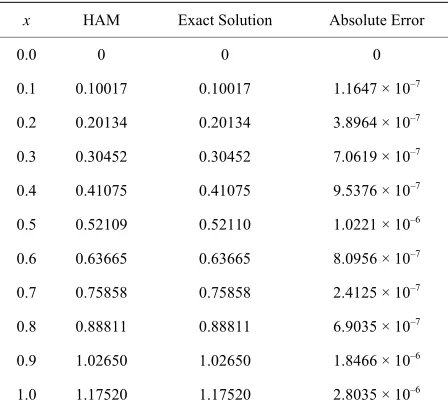
with the 10-term HAM approximate solution, and the numerical results can be seen in Table 1.
As mentioned in Section 2, the optimal value of is
de he
also
h
o t termined by the minimum of 7, corresponding t nonlinear algebraic Equation d7 = 0. Our c
dh
showed that, 7
alculations
has its minimum value at 1.
5. Conclusion
In this paper, have successfully develop solving variat al problems. It is apparent
,we ed HAM for
ion ly seen that
werful and efficient technique in find-tions for wide classes of linear and HAM is a very po
ing analytical solu
0 0.2 0.4 0.6 0.8 1 0
0.2 0.4 0.6 0.8 1 1.2 1.4
x
y(x)
[image:8.595.61.286.85.264.2]HAM Exact
Figure 11. Comparison between the 10-term HAM so and the exact solution.
Table 1. The result of the HAM for n = 7 and h = –1. lution
x HAM Exact Solution Absolute Error
0.0 0 0 0
0.
0
0.30452 0.30452 7.0619 × 10⁻⁷
1 0.10017 0.10017 1.1647 × 10⁻⁷
0.2 .20134 0.20134 3.8964 × 10⁻⁷
0.3
0.4 0.41075 0.41075 9.5376 × 10⁻⁷
0.5 0.52109 0.52110 1.0221 × 10⁻⁶
0.6 0.63665 0.63665 8.0956 × 10⁻⁷
0.7 0.75858 0.75858 2.4125 × 10⁻⁷
0.8 0.88811 0.88811 6.9035 × 10⁻⁷
0.9 1.02650 1.02650 1.8466 × 10⁻⁶
1.0 1.17520 1.17520 2.8035 × 10⁻⁶
ob ed. ults got e perfor
ove at oblems, wa fied t
of M l case r to num
PM, VIM and ADM.
V. Fomin, “Calculus of Variations,” Prentice Hall, New Jersey, 1963.
[2] L. Elsgolts, “ nd the Calculus of
Variations,” M 77.
Journal of the
16-0032(75)90199-4
tain The res from th mance of HAM
tio r vari
HA
ional pr in specia
s speci is simila
hat the solu erical results of
n
H
REFERENCES
[1] I. M. Gelfand and S.
Differential Equations a ir Publisher Moscow, 19
[3] L. Elsgolts, “Calculus of Variations,” Pergamon Press, Oxford, 1962.
[4] C. F. Chen and C. H. Hsiao, “A Walsh Series Direct Method for Solving Variational Problems,”
Franklin Institute, Vol. 300, No. 4, 1975, pp. 265-280.
doi:10.1016/00
[5] M. Razzaghi and M. Razzaghi, “Fourier Series Direct Method for Variational Problems,” International Journal of Control, Vol. 48, No. 3, 1988, pp. 887-895.
doi:10.1080/00207178808906224
[6] M. Dehghan and M. Tatari, “The Use of Adomian De-composition Method for Solving Problems in Calculus of Variations,” Mathematical Problems in Enginee
pp. 653-679.
ring, 2006,
0.1016/j.physleta.2006.09.101
[7] M. Tatari and M. Dehghan, “Solution of Problems in Calculus of Variations via He’s Variational Iteration Method,” Physics Letters A, Vol. 362, No. 5-6, 2007, pp.
401-406. doi:1
1.
[8] O. Abdulaziz, I. Hashim and M. S. H. Chowdhury, “Sol- ving Variational Problems by Homotopy Perturbation Method,” International Journal for Numerical Methods in Engineering, Vol. 75, No. 6, 2008, pp. 709-72
doi:10.1002/nme.2279
[9] S. J. Liao, “The Proposed Homotopy Analysis Technique for the Solution of Nonlinear Problems,” Ph.D. Thesis, Shanghai Jiao Tong University, Shanghai, 1992.
[10] S. J. Liao, “Beyond Perturbation: Introduction to the
hod for
02)00790-7
Homotopy Analysis Method,” CRC Press, Chapman & Hall, Boca Raton, 2003.
[11] S. J. Liao, “On the Homotopy Anaylsis Met Nonlinear Problems,” Applied Mathematics and Compu-tation, Vol. 147, No. 2, 2004, pp. 499-513.
doi:10.1016/S0096-3003(
o. 2, 2005, pp.
8
[12] S. J. Liao, “Comparison between the Homotopy Analysis Method and Homotopy Perturbation Method,” Applied Mathematics and Computation, Vol. 169, N
618-634. doi:10.1016/j.amc.2004.10.05
[13] S. J. Liao, “Homotopy Analysis Method: A New Ana-lytical Technique for Nonlinear Problems,” Communica-tions in Nonlinear Science and Numerical Simulation,
Vol. 2, No. 2, 1997, pp. 95-100.
doi:10.1016/S1007-5704(97)90047-2
[14] T. Hayat, T. Javed and M. Sajid, “Analytic Solution for Rotating Flow and Heat Transfer Analysis of a Third- Grade Fluid,” Acta Mechanica, Vol. 191, No. 3
pp. 219-229.
-4, 2007,
0451-y
doi:10.1007/s00707-007-[15] S. Abbasbandy, “Soliton Solutions for the 5th-Order KdV Equation with the Homotopy Analysis Method,” Nonlin-ear Dynamics, Vol. 51, No. 1-2, 2008, pp. 83-87.
doi:10.1007/s11071-006-9193-y
[16] S. P. Zhu, “An Exact and Explicit Solution for the Valua-tion of American Put OpValua-tions,” Quantitative Finance, Vol.
6, No. 3, 2006, pp. 229-242.
doi:10.1080/14697680600699811
od,” Asian-European
Jour-0018-3
[17] S. Effati and H. Saberi Nik, “Analytic-Approximate Solu-tion for a Class of Nonlinear Optimal Control Problems by Homotopy Analysis Meth
nal of Mathematics, in press.
[18] J. H. He, “Homotopy Perturbation Technique,” Computer Methods in Applied Mechanics and Engineering, Vol.
178, No. 3-4, 1999, pp. 257-262.
[image:8.595.59.283.322.526.2]py Analysis Method,” 9, 2007, pp. 8403-[19] K. Yabushita, M. Yamashita and K. Tsuboi, “An Analytic
Solution of Projectile Motion with the Quadratic Resis-tance Law Using the Homoto
Journal of Physics A, Vol. 40, No. 2 8416. doi:10.1088/1751-8113/40/29/015
[20] L. N. Zhang and J. H. He, “Homotopy Perturbation Method for the Solution of the Electrostatic Potential Differential Equation,” Mathematical Problems in Engineering, 2006,